HEC-RAS 2D Flow Area Modeling

HEC-RAS 2D flow modeling can be used in a variety of different situations:

To develop a 2D flow area model, an understanding of how the 2D flow model works is required. This article covers the basics of 2D flow modeling.

HEC-RAS 2D Computational Methods

HEC-RAS provides four methods for computing the flow field in a 2D mesh, each of which may be selected from the Unsteady Flow Computational Options dialog box available from the Analysis ribbon menu.
2D computational options

Because the user can easily switch between the 2D computational solvers, each solver can be tried for a given model to see if the Shallow Water Equations (also known as Full Momentum equations) provides additional detail over the Diffusion Wave equations.

In total, HEC-RAS has four equation sets that can be used to solve for the flow moving over the computational mesh, as listed below:

Refer to this article in our knowledge base to learn more about the Unsteady Flow Computational Options command.

2D Diffusion Wave Computational Method

The 2D Diffusion Wave computational method is the default solver and allows the computations to run faster and with greater stability. Most 2D modeling situations, such as flood modelling, can be accurately modeled using this solver, where inertial forces tend to dominate frictional and other forces.

The Diffusion Wave computational method can be used in the following situations:

2D Full Momentum Computational Method

The 2D Full Momentum computational method (Shallow Water Equations), often referred to as the Saint Venant equations for shallow flow, can account for turbulence and Coriolis effects, making it applicable to a wider set of conditions. However, solving the 2D Saint Venant flow equations requires more computational power and thereby results in longer run times. In addition, the 2D Saint Venant flow equations can become numerically unstable in regions of the 2D mesh where the water surface profile or flow direction is changing rapidly. To avoid an unstable model, a finer mesh and a corresponding smaller time step will need to be used.

The Shallow Water Equations should be used for greater accuracy in several applications. A general approach is to use the Diffusion Wave equations while developing the model. Once the model is working, the user can develop a different scenario and use the Shallow Water Equations to compare the results. A significant difference in results means the Shallow Water Equations solution is more accurate.

The new SWE-Eulerian Method is an explicit solution scheme that is based on a more conservative form of the momentum equation. It produces less numerical diffusion than the original SWE equation. However, in general, the SWE-Eulerian Method is only needed when users are interested in taking a very close look at changes in water surfaces and velocities at and around hydraulic structures, piers/abutments, and tight contractions and expansions. The original SWE-Eulerian-Lagrangian Method is more than adequate for most problems requiring the full momentum equation-based solution scheme. The SWE Local Inertia Method is a simplified version of the SWE equations. It is computationally more efficient. This method neglects the advection, diffusion, and Coliolis terms in the momentum equation, which results in a system of equations that is much simpler to solve..

The Full Momentum computational method should be used in the following situations:

Hotstart (or Restart) Initial Conditions

Because the 2D Diffusion Wave computational method runs much faster than the 2D Full Momentum computational method, the Diffusion Wave computational method can be used to create a hotstart (or restart) file to setup the initial conditions for the 2D mesh. The Full Momentum computational method can then use the hotstart file to define the initial water surface elevations and flows throughout the 2D mesh and then analyze the actual flood event.

2D Implicit Finite Volume Solution Algorithm

Both the 2D Diffusion Wave and 2D Saint Venant solvers use an implicit Finite Volume solution algorithm. The implicit solution method allows for larger computational time steps than explicit solution methods. In addition, the Finite Volume method provides a greater degree of stability and robustness over traditional Finite Difference and Finite Element methodologies.

The 2D computational process is as follows:

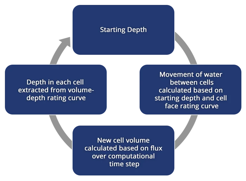Steps used in computing the flow through each cell in HEC-RAS 2D solver

This computational algorithm is very robust and allows 2D cells to wet and dry. 2D flow areas can start completely dry and can handle a sudden rush of water into them. In addition, this algorithm can handle flow regimes that change with time:

HEC-RAS 2D Modeling Guidance and Assumptions

For the HEC-RAS 2D computational methodology, the following modeling guidance and assumptions are provided:

With HEC-RAS current limitations on modeling 2D pressure flow and road overflow at a bridge, the following methods can be used to model the bridge in a 2D flow situation:

2D Computational Time Step Selection

While developing a 2D model, computational runtime may need to be considered—depending upon the size of the model. The following factors can impact computational runtime:

For an initial run, a coarse time step can be used (e.g., 5 minutes) to see how the model behaves and performs.

To further refine the computational results, HEC-RAS provides an adjustable time step option, where the computational engine dynamically recomputes the required time step during the simulation based upon the Courant number specified.

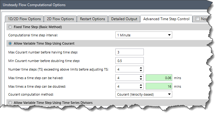
Adjustable time step option

An advantage of the variable time step option is that when not much flow change is occurring in the model, the software will speed up the computations by automatically selecting a larger time step. Then, when the flow conditions start to suddenly change (e.g., dam failure, levee overtopping, etc.), the software will automatically reduce the time step to capture this change. Overall, the variable time step option can provide significant savings in computational time.

Courant numbers as high as 3.0 can be used when the Full Momentum computational method is selected, while Courant numbers as high as 5.0 can provide enough accuracy and stability when using the Diffusion Wave computational method.

However, there may be instances where a Courant number of 1.0 (or less) is required for accuracy and stability—even when using the more stable Diffusion Wave method. Generally, the computation interval should be small enough such that the time required for water to move through any cell is greater than the time step interval. Most importantly, the time step selected must be sufficiently small to produce stable results, which can be determined by viewing stage and discharge hydrograph plots from within the 2D mesh.

Refer to this article in our knowledge base to learn more about the Unsteady Flow Computational Options command.

2D Computational Output Settings

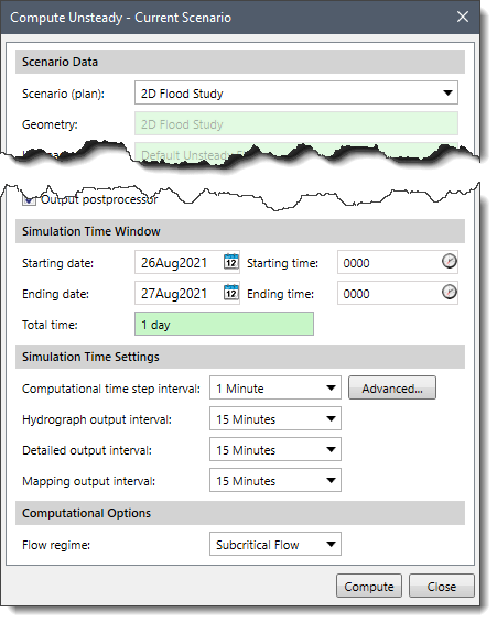
As discussed in the prior section, many items can impact the computational run times. An area that is commonly overlooked is the output interval specified in the Compute Unsteady – Current Scenario dialog box.

2D computational output settings

2D Computational Volume Accounting

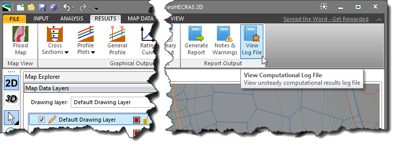
After the simulation has run, the user can check the computational results to determine if the conservation of mass (volume) was maintained during the simulation. From the Results ribbon menu, select the View Log File menu item.

View the computational log file for the volume accounting

This will display a text window showing the results. Scroll to the bottom of the listing to see the overall volumetric percent error in the 2D computations. Generally, this value should be less than 2 percent, and with additional model tuning (as discussed in this article) the percent error can be reduced even more—as shown in this example with 0.002185% error.

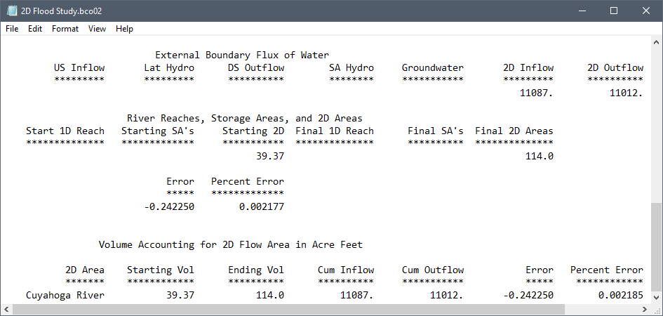
Computational log file

2D Flow Area External Boundary Conditions

2D flow areas are created by constructing polygon areas representing the regions to be modelled. Along the 2D flow area polygon mesh boundary, boundary condition polylines are defined to represent different flow conditions or constraints that are to be applied to the 2D flow area. These boundary conditions represent flux boundaries, where flow enters or leaves the 2D flow area. (Boundary conditions can also be defined within the interior of the 2D flow area, to represent additional discharge that enters the 2D flow area—such as flow from a wastewater treatment plant.)

Examples of flux boundaries are:

The polygon edges where no boundary conditions are defined are called slip boundaries. These boundaries basically act as frictionless, infinitely tall “glass” walls. 2D flow that encounters a slip boundary will be contained within the 2D flow area, like the vertical sides of a drinking glass.

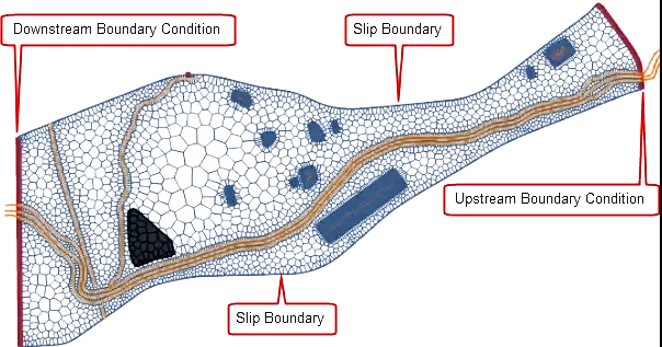
Different 2D flow area boundary types

2D Flow Area Internal Boundary Conditions

Additional flow can be introduced into the 2D flow area interior. Use the Assign SA/2D Boundary Condition Lines or Draw SA/2D Boundary Condition Lines command to add a boundary condition line to the interior of the 2D flow area.

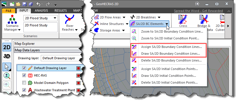
Drawing and Assigning boundary conditions to the 2D mesh

An internal boundary condition line must lie completely within the 2D mesh. It cannot be shared with the exterior boundary of the 2D flow area.

Refer to this article in our knowledge base to learn more about drawing and assigning SA/2D boundary condition lines.

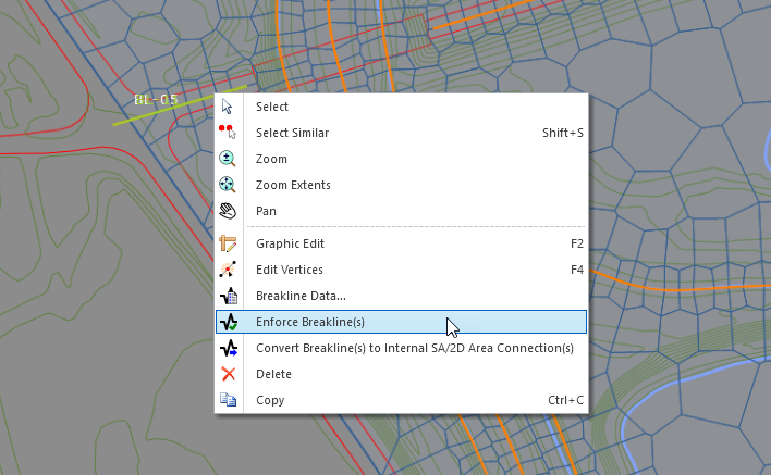
After adding the 2D boundary condition to the interior of the 2D mesh, the mesh faces need to be aligned with the defined boundary condition line. Select the 2D boundary condition polyline and then right-click. Select Enforce Breakline(s) option from the displayed context menu.

Only flow hydrographs with positive or zero values can be assigned as an internal boundary condition. Negative flow values are not allowed. In addition, pumps can be connected to a 2D mesh cell. To extract flow from the interior of a 2D flow area, such as for a water supply pump, an internal connection can be defined (described in the next section) along with a rating curve or time series representing the extraction rate.

2D Flow Area Internal Connections

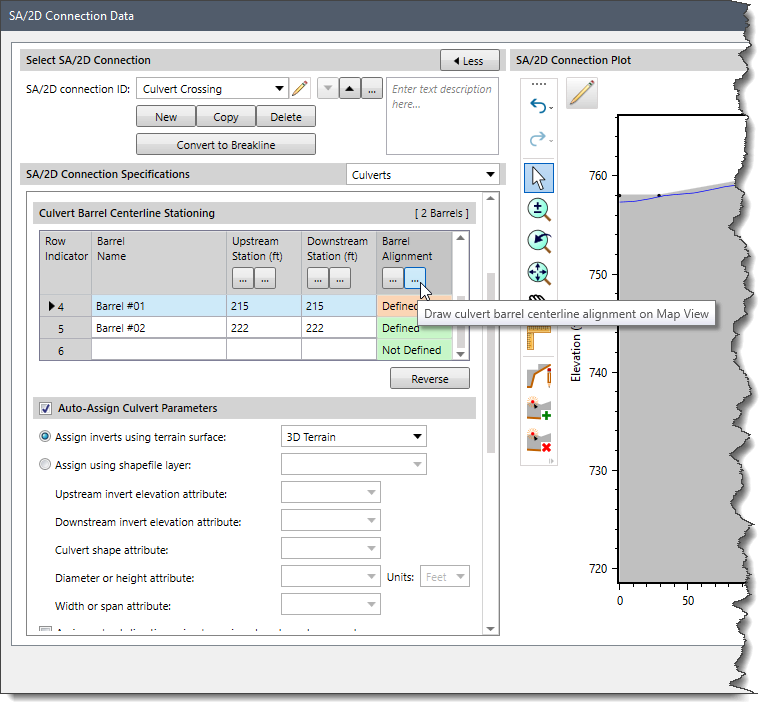
It is not uncommon to see unreasonable results at dams during a 2D simulation, including erroneously high-water surface elevations due to a lack of release from the dam. This is generally due to the orientation of 2D mesh cells. In such cases, spillways, gates and culvert openings can be incorporated within the 2D flow area using a SA/2D connection representing the dam. The SA/2D Connection Data dialog box is used to define these structures.

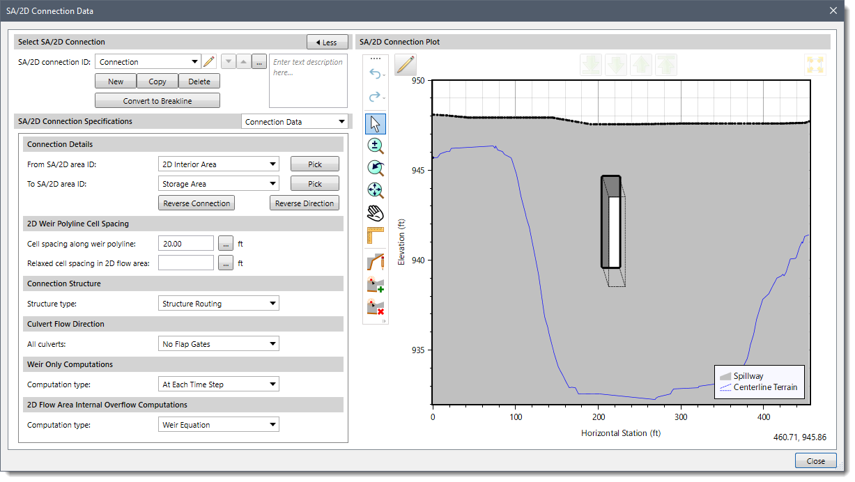
SA/2D Connection Data dialog box used to define connections to and within 2D flow areas

The internal connection weir geometry can be used to represent the dam crest and spillway geometry. When using internal connections, the weir flow equations might cause instability and smaller time steps may be required to model the weir flow over the dam and spillway structure. However, for internal connections along dams and other features that behave as weirs, the weir equations should be examined for the model.

2D Flow Area Elements

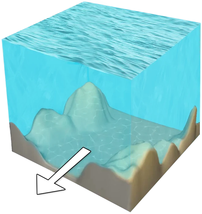
The 2D mesh cells consider the underlying ground terrain by creating geometric and hydraulic property tables that represent the elevation versus storage volume of the cell and the elevation versus flow area for each of the cell faces. Unlike other 2D flow models, HEC-RAS 2D flow area element cells do not have a flat bottom or a single depth. Therefore, a cell can be partially wet with the correct water volume for a given water surface elevation. Similarly, each of the cell faces are treated like a cross section where detailed hydraulic property tables are computed for elevation versus flow area, wetted perimeter, roughness, etc. This allows larger 2D cells to be used in the HEC-RAS flow computations without losing too much of the underlying terrain details that govern the movement of flow.

Idealized representation of a computational 2D cell used by the HEC-RAS 2D solver

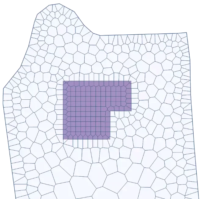
Because larger cells can be used in a HEC-RAS 2D flow model in comparison with other 2D flow models, it is important that cell faces be aligned with controlling terrain features, such as river centerlines, bank lines, roadways and levees in order to capture the hydraulic behavior of the 2D flow. Because larger cells can be used, the result is fewer computations, which directly translates into faster computational time.

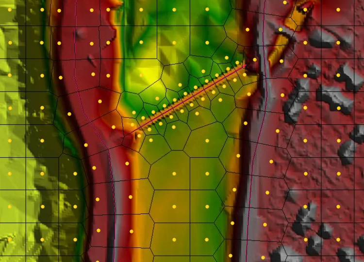2D computational mesh with breaklines aligned to control terrain features

The above figure shows the computational mesh over elevation color-shaded terrain data. The cell centers are where the water surface elevation is computed for each cell. The elevation-volume relationship for each cell is based on the surface geometry of the underlying terrain. Each cell face is represented internally with a detailed cross section based on the underlying terrain.

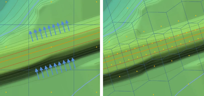
Flow of water between cells is based on the details of the underlying terrain, as represented by the cell face geometry and the volume contained within that cell. Hence, a small channel that cuts through a cell, and is much smaller than the cell, is still represented by the cell’s elevation-volume relationship and the hydraulic properties of the cell faces. This means water can run through larger cells but still be represented with its normal channel properties.

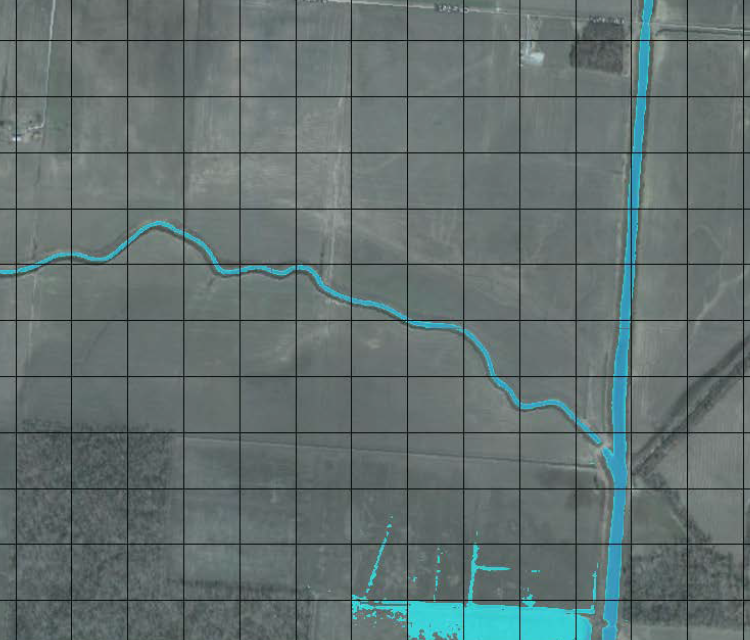Performing detailed hydraulic modeling with larger cells

An example of a small channel running through much larger grid cells is shown above. In this example, there are several channels that are much smaller than the cell size used to model the area. The cells are 500 ft square, and the channels are less than 100 ft wide. As shown, flow can travel through the smaller channels using the channel’s hydraulic properties. Flow remains in the channels until the river stage is higher than the bank elevation of the channel, where it then spills out into the overbank areas.

2D Flow Area Mesh Types

GeoHECRAS can create the following 2D mesh types. However, HEC-RAS can only create 2D uniform meshes (i.e., square and rectangular elements).

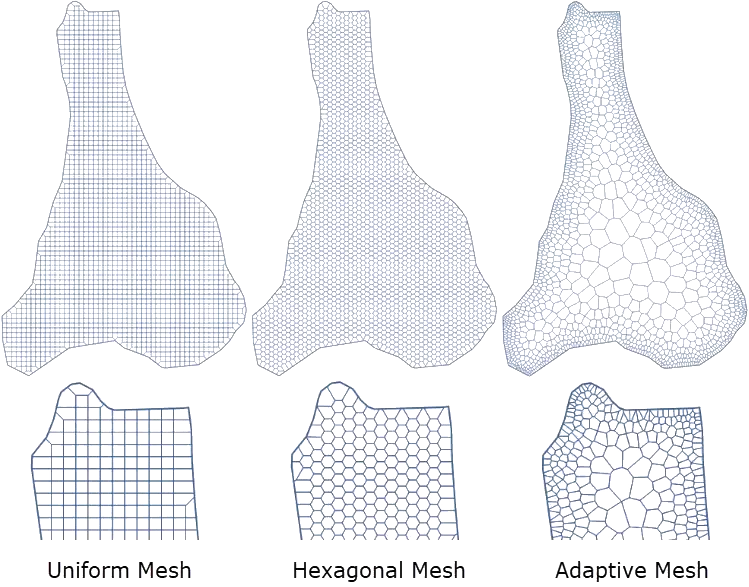
Each of the above mesh types have their own advantages and disadvantages. Each of these different mesh types can be incorporated within a single 2D flow area using zonal meshing—as described in a later section.

HEC-RAS Uniform 2D Mesh

HEC-RAS can create a mesh that contains squares and rectangles, although only square elements are created in practice. GeoHECRAS simplifies the process of defining these mesh elements by always creating square-shaped elements. Where breaklines are defined, the HEC-RAS meshing engine will refine the mesh using irregular mesh elements so that the mesh cell faces align with the breaklines.

Part of the difficulty with a uniform mesh is that all the cells throughout the entire mesh are the same size. Therefore, when there are regions where a refined mesh is necessary, there is not an automated way of refining the mesh (i.e., creating smaller cells). Similarly, where there are regions where the mesh cell sizes could be larger, there is not an automated way of relaxing the mesh (i.e., creating larger cells).

HEC-RAS Hexagonal 2D Mesh

Similar to the uniform mesh, a hexagonal mesh creates cells that are 6-sided and of uniform size. This mesh type is a bit better at modeling changes in flow direction since the cell faces are generally perpendicular to any flow entering or leaving the cell. However, this mesh type faces issues similar to that of a uniform mesh, as previously described.

HEC-RAS Adaptive 2D Mesh

For a large and complex 2D flow study area, an adaptive 2D mesh can be used in place of a 2D uniform (i.e., square cells) or 2D hexagonal mesh for a faster and more accurate simulation. Adaptive 2D meshing allows GeoHECRAS to determine what size and shape element should be used, based upon the underlying terrain elevation change and user-defined breaklines. Generating a 2D adaptive mesh takes slightly longer than generating a 2D uniform mesh because of the additional computations that the software performs in creating the mesh while it sizes and shapes the 2D elements. The completed 2D adaptive mesh will have automatically refined elements (i.e., creating smaller elements) in areas where additional detail is required, and relaxed elements (i.e., creating larger elements) in areas where the 2D flow is relatively uniform and not much change is occurring. Because of the inherent advantages of the 2D adaptive mesh, the HEC-RAS 2D flow simulations tend to be more stable (because of smaller element sizes where sudden changes occur) and run quicker (because of smaller total number of elements) than an equivalent 2D uniform mesh.

Mesh Editing

While creating a 2D flow area mesh, it may become necessary to manually edit the mesh. Several mesh editing tools are provided in the 2D Flow Area Preview section of the 2D Flow Area Data dialog box.

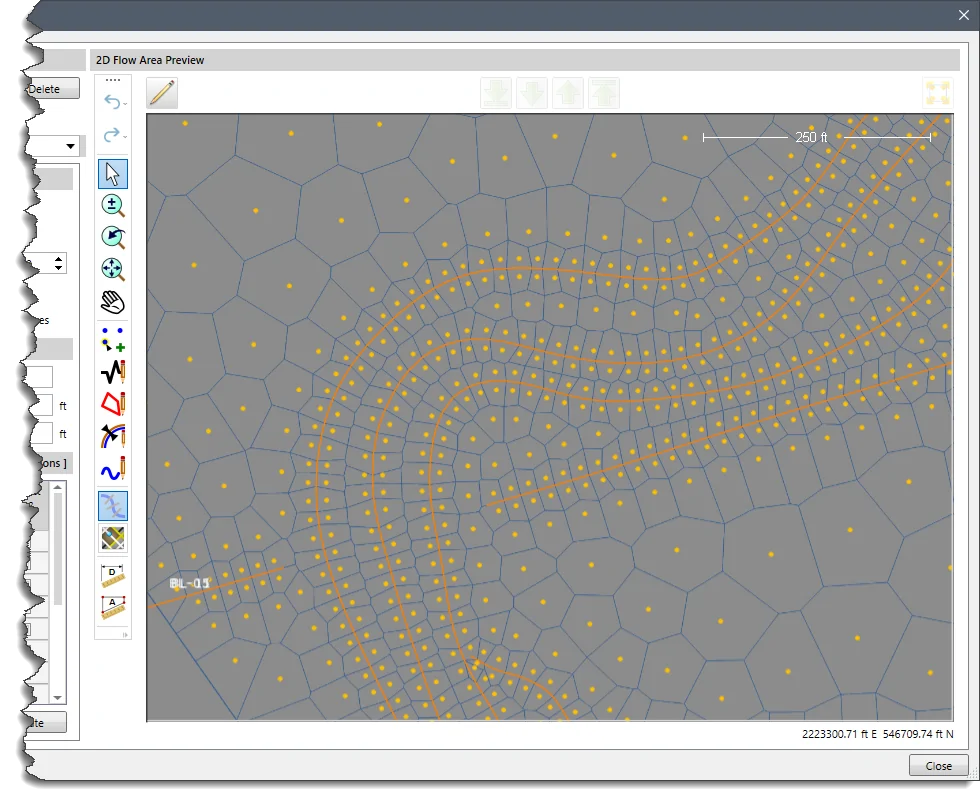
Several mesh editing tools are provided

The following tools and editing commands are provided within the 2D Flow Area Data dialog box as well as from the Map View.

In addition, unlimited undo and redo functionality is provided for all mesh editing commands.

Mesh Development Guidelines

Problematic sharp angles should be avoided when defining the mesh boundary and defining breaklines and other mesh controlling elements (i.e., 2D connections, 2D conveyance obstructions, etc.). If jagged edges exist for a 2D mesh boundary or breakline, significant mesh modifications will be required. Not performing this step could be the difference between minutes versus a day when creating an error-free HEC-RAS 2D mesh.

It is recommended that 2D mesh errors be addressed by first modifying the mesh boundary and breaklines, as opposed to moving mesh cells. Using this approach should help eliminate the need to resolve repeated errors regarding cells along the mesh boundaries and breaklines that would occur when a new mesh is generated (such as if a new cell size is defined).

Mesh Generation – Rebuild and Update Commands

After the user has added additional 2D elements, breaklines, 2D connections, 2D mesh zones, 2D bridge piers, and more, the 2D flow area mesh needs to be updated to include these features and mesh changes. The Rebuild and Update commands in the 2D Flow Area Data dialog box can be used for updating the 2D flow area mesh.

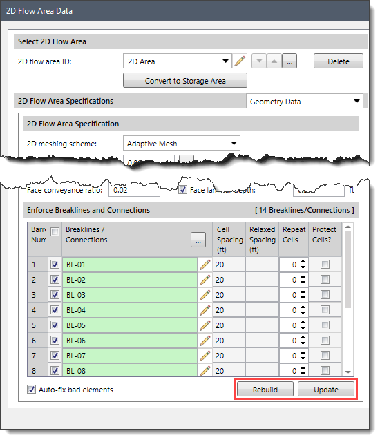
The Rebuild and Update commands will cause the software to recreate the 2D flow area mesh

Descriptions of these commands follow:

Rebuild Command

This command causes the software to recreate the entire 2D mesh using all the defined features. Any user edits to the 2D mesh elements are discarded.

Update Command

This command is like the Rebuild command but retains all user edits to the 2D mesh elements. This is helpful because the user may have performed several manual refinements and edits to the 2D mesh and using this command will cause the mesh generation to include all of these refinements and edits.

Notes:

Automatic Correction of 2D Mesh Bad Elements

The HEC-RAS automated 2D mesh generation feature works well but can create meshes that have the following problems.

HEC-RAS requires that the user manually edit the problematic cells, whereas GeoHECRAS will automatically correct these bad cells. To direct GeoHECRAS to correct these bad cells, make certain that the Auto-fix bad elements check box is checked in the 2D Flow Area Data dialog box.

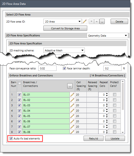
Auto-fix bad elements option will cause the software to correct any malformed 2D elements

Refer to this article in our knowledge base for more information on potential mesh generation problems.

2D Flow Area Zonal Meshing

To take advantage of the various 2D mesh types that GeoHECRAS provides, the software allows the user to define mesh zones within a 2D flow area, where each zone can have its own mesh type and corresponding parameters (e.g., element size, etc.). This allows the user to define refinement regions for specific areas of interest. For example, in a critical infrastructure area, a mesh zone could be defined, and a much smaller element size used to capture the flow direction and velocities that occur during a flood event.

Zonal Meshing

2D Flow Area Breaklines

Breaklines are used to define sudden breaks in the terrain surface and where interruptions in surface water flow will occur. Breaklines should be added where there is:

Breaklines force the 2D mesh cell faces to align with the breakline and prevent cells from crossing the breakline. Breaklines are critical to creating an accurate 2D mesh, so that the mesh properly represents an accurate bathymetric model.

When defining a breakline, the user can specify the cell size (or cell spacing) along the line. This can be used to refine the 2D mesh where additional detail needs to be captured in the defined model—such as along a stream or river channel. Breaklines can be used along, and be offset from, elevated roadways and other obstructions to flooding to sculpt the mesh to incorporate these features into the model.

Creating a 2D mesh is often an iterative process, where the modeler revises the 2D mesh to represent the 2D flow characteristics for the region being modelled. Hence, breaklines can be added at any time to the 2D mesh. When drawing breaklines, align them with levees, roads, and any high ground that you want the mesh faces to align with. Breaklines should be placed along the main channel banks in order to keep flow in the channel and until the flow gets high enough to overtop any high ground along the main channel.

When cell edges are situated along the crest of roadway embankments, flow through the obstruction is prevented and instead retained behind these embankments, as dictated by the surrounding topography. The cell size along the breaklines should be defined small enough to model the conveyance being routed along a roadway ditch, etc. Culverts and other roadway crossings can be modeled using SA/2D connections, allowing flow to pass through the roadway embankment to the other side of the roadway.

If an elevation feature, such as a roadway embankment that would impede flow, lies within a grid cell instead of along a cell edge, water will flow across that elevation feature before it gets high enough to overtop that elevation feature. Adding a breakline along the top of the elevation feature will correct this issue, as shown below.

Example of flow jumping through an obstruction when large 2D flow cells are used

Breaklines should be placed along a dam crest, and the cell size for such breaklines may need to be set finer than the nominal 2D mesh cell size. Breaklines along dams can also be converted to internal connections, for which the weir geometry can be used to represent the dam.

After performing an initial simulation, it should become clear where significant trouble spots exist, creating artificial backwater. Care should be taken to refine the 2D mesh at these locations to ensure the mesh accurately represents how the flow travels. A balance between refining the mesh in trouble spots to produce satisfactory results and unnecessary mesh editing is obvious; the point of diminishing returns should be relatively easy to identify after a first pass of refining significant trouble areas. If there are numerous small structures in the area being modeled, defining them using breaklines or internal connections may be hydraulically insignificant and should be avoided.

When using breaklines to account for levees, roadway embankments, and other features that act like levees, consideration should be taken to only apply breaklines where the feature provides realistic flood protection. Modeling non-FEMA accredited levees may produce unreasonable results representing flood protection that really does not exist. Therefore, engineering judgement should be used when defining breaklines for levees and levee-like features.

GeoHECRAS allows you to assign breaklines from previously defined CAD or GIS polylines, or by interactively drawing them on the Map View. From the Input ribbon menu, select the 2D Breaklines menu. You will see commands for assigning or drawing a breakline.

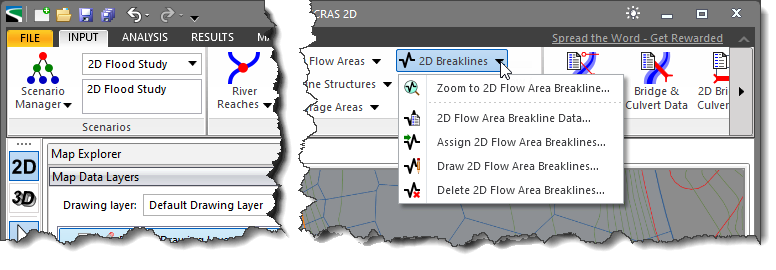
Input ribbon menu contains several commands for creating and editing breaklines

The Assign 2D Flow Area Breaklines and Draw 2D Flow Area Breaklines commands have similar dialog boxes, as shown below. The software will automatically name the breaklines, but the user can change the name to whatever is desired.

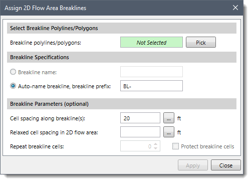
Assign 2D Flow Area Breaklines dialog box

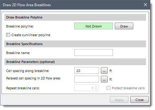
Draw 2D Flow Area Breaklines dialog box

The following entries are used to control how 2D cells are created in the vicinity of the breakline:

Cell Spacing along Breakline

This entry represents cell spacing along the breakline. If this entry is left blank, then the cell spacing used in the vicinity of the breakline will be used. Click on the […] button to measure the cell spacing from the Map View.

Relaxed Cell Spacing in 2D Flow Area

This entry represents the cell spacing further away from the breakline. If this entry is left blank, then the cell spacing used in the vicinity of the breakline will be used. This value should not be the same as the Cell spacing along breakline value, or there may be many cell errors introduced along the breakline. Click on the […] button to measure the cell spacing from the Map View. When creating the mesh, the software will automatically gradually transition the cell size from what is defined for the breakline and the area surrounding the breakline.

Breakline Context Menu

Right-clicking on the breakline will display a context menu. This menu contains commands that are specific to the selected breakline. For example, the Enforce Breakline(s) context menu command will cause the software to regenerate the mesh in the vicinity of the breakline so that the cell faces align with the breakline. Note that some bad elements may be reported after enforcing the breakline into the mesh. However, the software will automatically fix these bad elements when the mesh is rebuilt from within the 2D Mesh Area Data dialog box, as described in this article.

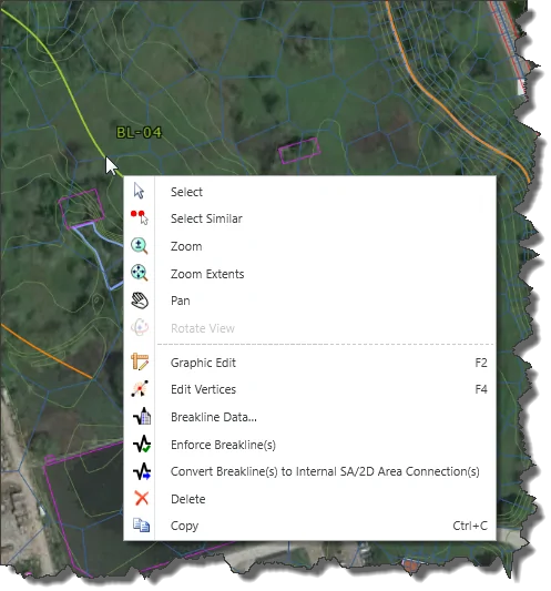Right-click context menu for breaklines

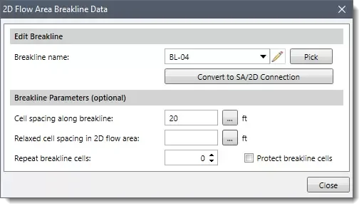
Double-clicking on a breakline will cause the 2D Flow Area Breakline Data dialog box to be displayed. This dialog box provides some additional information that can be used to define how the breakline influences the 2D mesh.

2D Flow Area Breakline Data dialog box

The following additional entries control how 2D cells are created in the vicinity of the breakline:

Repeat Breakline Cells

This spin control causes additional layers of identically sized cells to be created adjacent to the breakline cells.

Protect Breakline Cells

This checkbox causes the software to leave any manual edits of the cells that align with the breakline as they are. Regenerating the 2D mesh will not change the cells that are adjacent to the breakline.

The 2D Flow Area Data dialog box also allows the user to edit the breakline data. The Enforce Breaklines and Connections section allow the user to edit some of the breakline data, as well as disable breaklines that are already defined.

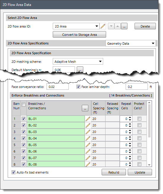
Breakline section contained within the Geometry Data panel of the 2D Flow Area Data dialog box

2D Ineffective Flow Areas

Ineffective flow areas can be assigned to the 2D mesh to account for regions where the water is not actively being conveyed. The water will pond in such areas, and its velocity in the downstream direction will be close to zero. These defined regions are included in the storage calculations but are not included as part of the active flow area. When using ineffective flow areas, no wetted perimeter friction is included at the boundary between the ineffective flow area and active flow area.

Ineffective flow at the entrance to a culvert

GeoHECRAS allows the user to define 2D ineffective flow areas using polygons. The software will automatically refine the 2D mesh to accommodate the ineffective flow area shape.

Refer to this article in our knowledge base for further discussion of 2D ineffective flow areas and how to create them.

2D Conveyance Obstructions

Conveyance obstructions can be assigned to the 2D mesh to account for regions that are permanently blocked from conveying flow. Conveyance obstructions, such as buildings and other structures, decrease the flow area and add additional wetted perimeter where the water comes in contact with the obstruction.

GeoHECRAS allows the user to define 2D conveyance obstructions using polygons. The software will automatically refine the 2D mesh to accommodate the conveyance obstruction shape.

Refer to this article in our knowledge base to learn more about 2D conveyance obstructions and how to create them.

2D Bridge Modeling

When working with bridges with complex geometry, modeling the hydraulics in 2D provides a clearer understanding and a more accurate representation of the flow behavior at the bridge. Water may flow through multiple paths and directions at the bridge opening. A HEC-RAS 1D model will assume that the water surface elevation is constant across the bridge opening, whereas a HEC-RAS 2D model will show that the water surface elevation varies across the bridge opening as the flow makes its way through the opening. In addition, a 1D model assumes an average velocity at the bridge opening, while a 2D model will accurately represent the velocity field at the bridge. This is particularly important when computing potential bridge pier scour. There are other drawbacks to using a HEC-RAS 1D model for bridge analysis:

The above concerns are automatically handled when using a 2D model. Many bridge modeling situations exist that are effectively managed with a 2D model, but that would be problematic with a 1D model. For example, modeling skewed bridges can cause additional energy losses and increased water surface elevations, conditions that would not be apparent when using a 1D model.

2D flow around bridge piers

GeoHECRAS provides additional functionality to speed up 2D modeling of bridges, including stamping of bridge piers directly into the 2D flow area mesh.

Refer to this article in our knowledge base to learn more about HEC-RAS 2D bridge modeling with GeoHECRAS.

2D Culvert Modeling

Culvert roadway crossings can be incorporated into a 2D flow area using internal connections. GeoHECRAS allows the user to draw the internal connection on the Map View, which is used to represent the roadway centerline (weir geometry). The culverts can also be drawn on the Map View, with the culvert invert elevations extracted from the terrain model or assigned from a corresponding GIS shapefile. The 2D flow area cells should be small enough so that the culvert inlet and outlet correspond to different cells. The culvert inlet and outlet cannot reside in the same 2D flow area cell.

Different tools and options are provided for assigning culverts in a 2D mesh

After creating the roadway crossing and culverts, the roadway geometry and culverts are shown on the Map View.

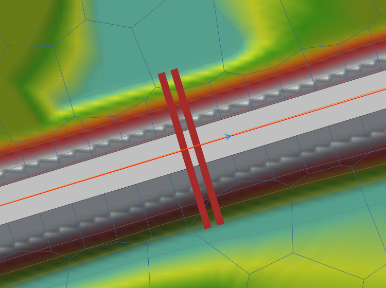Culvert alignments can be assigned or drawn in the 2D mesh

However, looking at the culvert inlet and outlet locations on the Map View, it may be necessary to refine the cells around the inlet and outlet. Use the Draw Breaklines command and place breaklines a short distance from the culvert inlet and outlet locations. Then update the mesh and culvert inlet and outlet locations to be well within a local cell. Alternatively, the user can use the 2D Flow Area Data dialog box and add and/or move 2D cells to develop a refinement. However, this requires that the user manually edit the cells at the culvert inlet and outlet each time the 2D flow area mesh is rebuilt.

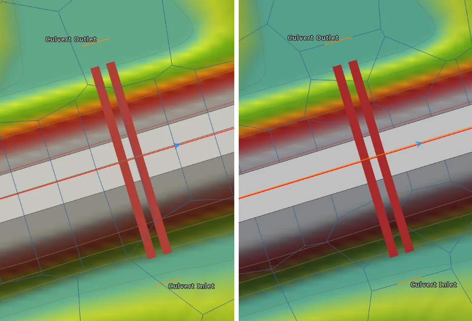Refining the 2D mesh at the culvert inlets and outlets

When defining culverts in a 2D flow area, the culvert inverts cannot be lower than the terrain elevation of the 2D cells in which the inlet and outlet are connected. Either the culvert inverts can be adjusted upward, or the Adjust Elevations command contained in the Terrain ribbon menu can be used to lower the cell elevations in which the culvert inlet and outlet are connected.

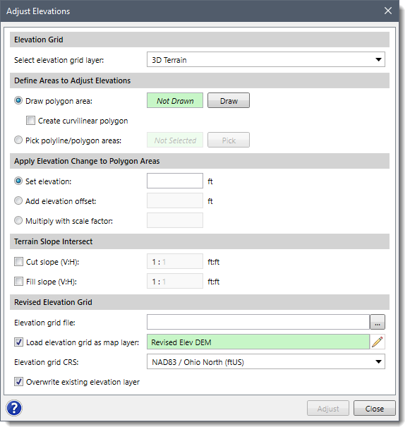
Adjust Elevations command can adjust the cell elevations at the culvert inlet and outlet.

Refer to this article in our knowledge base to learn more about the Adjust Elevations command.