1D/2D Flow Options

In GeoHECRAS, the 1D/2D Flow Options panel of the Unsteady Flow Computational Options dialog box allows the user to control the 1D unsteady flow calculation and mixed flow regime capabilities.
1D/2D Flow Options panel

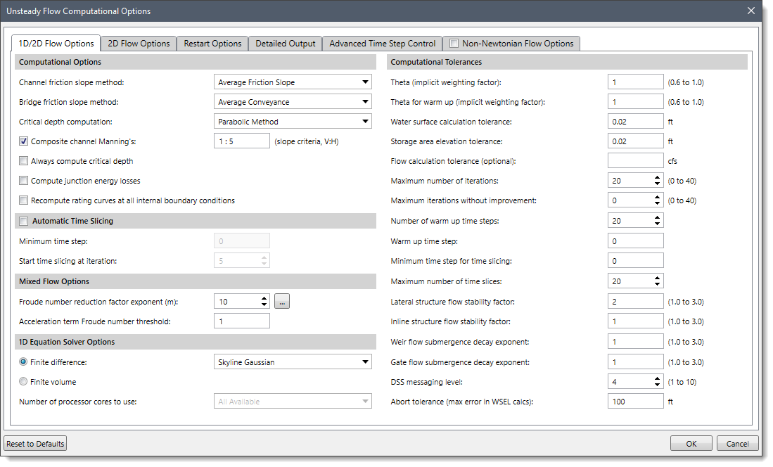
The following sections describe how to interact with the 1D/2D Flow Options panel of the Unsteady Flow Computational Options dialog box.

Computational Options

This section provides various options to select friction slope methods for channels and bridges, critical depth computation methods, and other runtime computational options.
Computational Options section

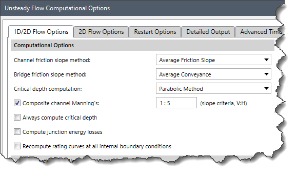
The following options are provided in the Computational Options section:

Channel friction slope method: This dropdown combo box allows the user to select one of six available friction slope methods. The six methods are as follows:
1. Automatic Selection
2. Average Conveyance
3. Average Friction Slope (default)
4. Geometric Mean
5. Harmonic Mean
6. HEC-6 Slope Averaging
Bridge friction slope method: This dropdown combo box allows the user to select one of six available slope averaging methods for computing frictional forces through bridges. The six methods are as follows:
1. Automatic Selection
2. Average Conveyance (default)
3. Average Friction Slope
4. Geometric Mean
5. Harmonic Mean
6. HEC-6 Slope Averaging
  
  By default, the software selects the Average Conveyance method. This method has been found to give the best results at bridge locations.

Critical depth computation: This dropdown combo box allows the user to select one of the following two available methods for calculating critical depth.
1. Parabolic Method: By default, the software selects this method. This method utilizes a parabolic searching technique to find the minimum specific energy. This method is very fast, but it can only find a single minimum on the energy curve.
2. Multiple Critical Depth: This method can find up to three minimums on the energy curve. If more than one minimum is found, the software selects the answer with the lowest energy.
  
  Note that the Multiple Critical Depth method takes a lot of computation time. Since critical depth is calculated often, using this method will slow down the computations. This method should only be used when you feel the software is finding an incorrect answer for critical depth.

Composite channel Manning’s: Checking this checkbox causes the software to composite all the main channel Manning’s n values into a single n value, as long as the side slopes of the main channel are greater than 1V:5H slope criteria. The user has the option to change this slope criterion. By default, this checkbox is checked.
Always compute critical depth: Checking this checkbox causes the software to calculate the critical depth at all locations. By default, this checkbox is unchecked.
Compute junction energy losses: Checking this checkbox causes the software to compute minor energy losses due to bends, junctions, etc. By default, this checkbox is unchecked.
Recompute rating curves at all internal boundary conditions: Checking this checkbox causes the software to recompute all internal boundary conditions. If left unchecked, the software will read in previously computed curves for internal boundary conditions like bridges, culverts, etc. By default, this checkbox is unchecked.

Automatic Time Slicing

This section allows the user to invoke time slicing when the maximum number of iterations is reached.
Automatic Time Slicing section

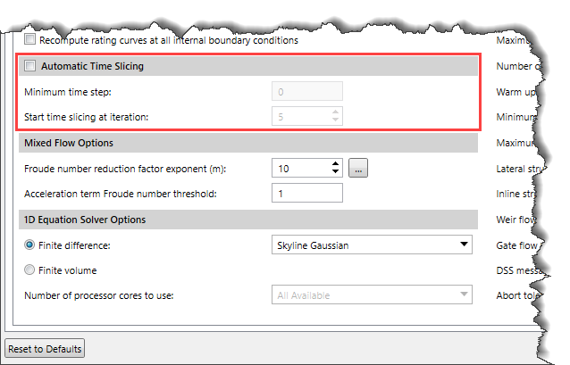
The user can select the Automatic Time Slicing checkbox to enable this section. After enabling this section, the user must define the minimum time step value (Minimum time step) and the iteration point at which time slicing will start (Start time slicing at iteration). Time slicing will be done to the point where the maximum iteration is reached.

Mixed Flow Options

This section is used for controlling the mixed flow regime capabilities used with the 1D Finite Difference solution scheme. It allows the software to run in such a mode that it will allow the 1D Finite Difference solution scheme to handle the subcritical flow, supercritical flow, hydraulic jumps, and draw downs (sub to supercritical transitions).
Mixed Flow Options section

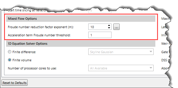
The software uses the Local Partial Inertia (LPI) solution technique for mixed flow regime analysis. The user can click the […] button to display a graphical plot displaying the magnitude of the LPI factor for a given Froude number and a given exponent ‘m’.
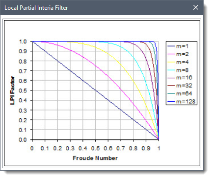
Local Partial Interia Filter window

The default values for the Froude number threshold and the exponent are FT = 1 and m = 10. The user can define different values for the Froude number threshold and the exponent in Acceleration term Froude number threshold and Froude number reduction factor exponent (m) fields.

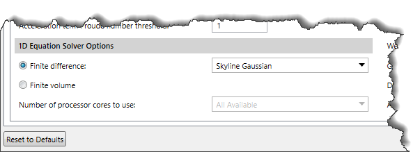
1D Equation Solver Options

This section allows the user to select a solution scheme for solving the 1D Shallow Water equations. The user can either use the 1D Finite Difference solution scheme or the 1D Finite Volume solution scheme. In addition, this section provides options to select the matrix equation solver for the 1D Finite Difference solution scheme and control the number of cores used to solve the problem.
1D Equation Solver Options section

The following options are provided:

Finite difference: Selecting this radio button option allows the user to use the 1D Finite Difference solution scheme to solve the 1D Shallow Water equations. The dropdown combo box adjacent to this option allows the user to select the matrix equation solver for the 1D Finite Difference solution scheme. Two options are available:
1. Skyline Gaussian (default)
2. Pardiso
  
  The Skyline Gaussian matrix solver is generally faster for dendritic river systems, whereas the Pardiso matrix solver may produce faster computational results for large, complex, and looped systems.

Finite volume: Selecting this radio button option allows the user to use the 1D Finite Volume solution scheme for solving the 1D Shallow Water equations.
Number of processor cores to use: This dropdown combo box gets enabled when the user selects the Pardiso matrix equation solver for the 1D Finite Difference solution scheme. The user can choose up to 64 processor cores to use for running the Pardiso By default, the software selects the All Available option.

Note that the speed of the solution is sensitive to the number of cores used, and it is not always faster to use the maximum number of cores available. So, the user should test the various options available for the number of cores to get the maximum computational speed benefit.

1D Finite Difference vs 1D Finite Volume Solution Scheme

The following table provides a comparison between the 1D Finite Difference and 1D Finite Volume solution scheme:

Finite Difference	1D Finite Volume
Cannot handle starting or going dry in a cross section (XS)	Can start with completely dry channels, or they can go dry during a simulation (wetting/drying)
Low flow model stability issues with irregular XS data	Very stable for low flow modeling
Cannot handle extremely rapidly rising hydrographs	Can handle extremely rapidly rising hydrographs without becoming unstable
Mixed flow regime (i.e., flow transitions)	Handles subcritical to supercritical flow and hydraulic jumps better – No special option to turn on
Stream junctions do not transfer momentum	Junction analysis is performed as a single 2D cell when connecting 1D reaches (continuity and momentum are conserved through the junction)

Generally, the 1D Finite Volume solution scheme is more robust (greater model stability) than the existing 1D Finite Difference solution scheme. However, there are some drawbacks to the new 1D Finite Volume solution scheme as listed below:

Users cannot use lidded cross sections with the new Finite Volume solution scheme: This also means that it cannot handle the pressurized flow, even with the Priessman slot option turned on. If the model contains lidded cross sections, as soon as the water hits the high point of the lids’ low chord, the model will become unstable.
The Finite Volume solution scheme is sensitive to the volume of water between any two cross sections: The equations are written from a “volume” perspective. If two cross sections are very close together, then there is very little volume between those two cross sections. The 1D Finite Volume scheme will require smaller time steps to handle the change in volume over the time step for this type of situation. The 1D Finite Difference scheme handles this better because the equations are written in terms of change in water surface and velocity, which may be a small change for cross sections that are closer together. Therefore, for the 1D Finite Volume scheme to work well with larger time steps, users may need to remove cross sections that are very close together.
The Finite Volume scheme is computationally slower than the Finite Difference solution scheme: This is because the Finite Difference scheme combined the properties of the left and right overbank together (area, wetted perimeter, average length between cross sections, etc.) and solved the equations for the main channel and a single floodplain. The new Finite Volume solution scheme keeps the left and right overbank properties separate. Thus, the equations are written for a separate left overbank, main channel, and right overbank, and then solved. This is more computational work for every time step, but it is computationally more accurate.
The Finite Volume Solver cannot be used with the Modified Puls Routing Option: The Modified Puls Routing option cannot be used with the Finite Volume solution scheme. This was done on purpose, as it was deemed users would not need the Modified Puls Routing option since the Finite Volume routing method can handle dry channels, extremely low flows, rapidly rising flows, and very steep channels. Modified Puls routing was added to HEC-RAS because the original Finite Difference solver has trouble in the areas previously described.

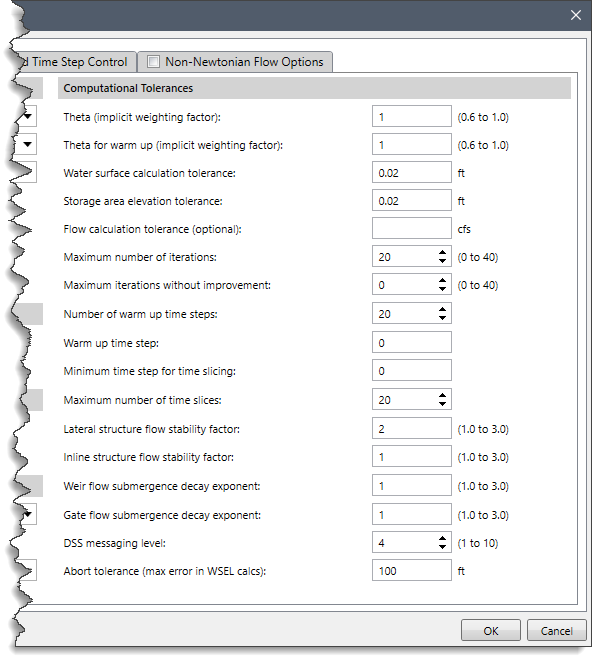
Computational Tolerances

This section provides various options to set the tolerances for unsteady flow equations.
Computational Tolerances section

The following options are provided to the user:

Theta (implicit weighting factor): This entry field is used to define the value of Theta (implicit weighting factor). This factor is used in the 1D Finite Difference solution scheme. The factor ranges between 0.6 and 1.0. A value of 0.6 will give the most accurate solution of the equations but is more susceptible to instabilities. By contrast, a value of 1.0 provides the most stability in the solution but may not be as accurate for some data sets. The default value for Theta is set to 1.0. Once the model is up and running the way users want it, they should then experiment with changing Theta towards a value of 0.6. If the model remains stable, then a value of 0.6 should be used.
Theta for warm up (implicit weighting factor): The unsteady flow solution scheme has an option to run what we call a warm up period (explained below). This entry field allows the user to set a different value for Theta during the warm up period versus the simulation period. By default, the software uses a value of 1.
Water surface calculation tolerance: This entry field allows the user to define the water surface calculation tolerance. This tolerance is used to compare the difference between the computed and assumed water surface elevations at cross sections. If the difference is greater than the tolerance, the software continues to iterate for the current time step. When the difference is less than the tolerance, the software assumes it has a correct numerical solution. The default value is set to 0.02 feet.
Storage area elevation tolerance: This entry field allows the user to define the storage area elevation tolerance. This tolerance is used to compare the difference between computed and assumed water surface elevations at storage areas. If the difference is greater than the tolerance, the software continues to iterate for the current time step. When the difference is less than the tolerance, the software can go on to the next time step. The default tolerance for storage areas is set to 0.02 feet.
Flow calculation tolerance (optional): This entry field allows the user to define the optional flow calculation tolerance. This tolerance is used to compare against the numerical error in the computed flow versus the assumed flow for each iteration of the unsteady flow equations. The user needs to enter a flow in cfs (or cms in metric units). The software monitors the flow error at all computational nodes. If the flow error is greater than the user entered tolerance, the software will continue to iterate. The flow calculation tolerance is only used if the user enters a value for the flow. By default, this field is left blank.
Maximum number of iterations: This field allows the user to define the maximum number of iterations the software will make when attempting to solve the unsteady flow equations using the specified tolerances. The default value is set to 20. The user can select any different value between 0 and 40.
Maximum iterations without improvement: This field allows the user to set a maximum number of iterations (0 to 40) in which the solver can iterate without improving the answer. Using this option can increase the speed of the computations but may cause more significant errors or instabilities to occur if not used correctly. A good starting value for this option would be 5. This means that if the analysis iterates five times and does not improve any of the solution errors, it will stop iterating at all nodes in the system and use the previous iteration that had the best answers up to that point. The premise here is that if the iteration scheme cannot improve the solution for five consecutive iterations, it is likely not going to improve, and there is no point in wasting computational time by iterating all the way to the maximum number of iterations.
Number of warm up time steps: This field allows the user to define the number of warm up time steps. Before the user-defined simulation period begins, the software can run a series of time steps with constant inflows. This is called a warm up period. The concept of warm up period is used to smooth the profile before allowing the inflow hydrographs to progress. This helps to make a more stable solution at the beginning of the simulation. By default, number of warm up time steps is set to 0. The user can select any value between 0 and 200.
Warm up time step: This entry field allows the user to define the time step value for the warm up period. During the warm up period, it is sometimes necessary to use a smaller time step than what will be used during the unsteady flow calculations. The initial conditions from the backwater analysis use a flow distribution in the reaches, which is often different than that computed by the unsteady flow. This can cause some instabilities at the beginning of the simulation. The use of a smaller time step during the warm up period helps to get through these instabilities. By default, the warm up time step value is set to 0. This means the software will use the time step that has been set for the unsteady flow simulation period.
Minimum time step for time slicing: The software can interpolate between time steps when it finds a very steep rise in an inflow hydrograph. This entry field allows the user to set a minimum time step to use when the software starts reducing time steps during a steep rise or fall in the flow at a boundary condition. It prevents the software from using too small of a time step during time slicing.
Maximum number of time slices: This field allows the user to define the maximum number of interpolated time steps that the software can use during time slicing. By default, the software uses a value of 20.
Lateral structure flow stability factor: This entry field allows the user to define the lateral structure flow stability factor. This factor is used to increase the stability of the numerical solution in and around a lateral structure. The factor varies from 1.0 to 3.0. As the value is increased, the solution is more stable but less accurate. A value of 1.0 is the most accurate but is susceptible to oscillations in the computed lateral flow. By default, the software uses a value of 2.0. If there are oscillations in the computed flow over a lateral structure, the user should first check to see if the used computational interval is small enough or not. If the computation interval is sufficiently small, the user should increase this coefficient to see if it solves the problem.
Inline structure flow stability factor: This entry field allows the user to define the inline structure flow stability factor. This factor is used to increase the stability of the numerical solution in and around an inline structure. This factor varies from 1.0 to 3.0. As the value is increased, the solution becomes more stable but less accurate. A value of 1.0 is the most accurate but is susceptible to oscillations in the computed flow. By default, the software uses a value of 1.0. If there are oscillations in the computed flow over the inline structure, the user should first check if the used computational interval is small enough or not. If the computation interval is sufficiently small, the user should increase this coefficient to see if it solves the problem.
Weir flow submergence decay exponent: This entry field allows the user to define the weir flow submergence decay coefficient. This coefficient is used to stabilize the solution of flow over a weir for highly submerged weirs. This factor varies from 1.0 to 3.0. As the headwater and tailwater stages become closer together, oscillations can occur in the solution. This exponent will prevent this from happening. The default value of 1 has no effect. On increasing the coefficient, dampening of the oscillations will occur.
Gated flow submergence decay exponent: This entry field allows the user to define the gated flow submergence decay coefficient. This coefficient is used to stabilize the solution of flow over a gated spillway for highly submerged flows. This factor varies from 1.0 to 3.0. As the headwater and tailwater stages become closer, oscillations can occur occasionally in the solution. This exponent will prevent this from happening. The default value of 1 has no effect. On increasing the coefficient, dampening of the oscillations will occur.
DSS messaging level: This field allows the user to control the amount and detail of messages written to the log file when reading and writing data to HEC-DSS. A value of 1 is minimal information, and a value of 10 turns on the maximum amount of information. By default, the software uses a value of 4.
Abort tolerance (max error in WSEL calcs): This entry field allows the user to set a maximum water surface error that will cause the analysis to stop running if it is exceeded. The default value is 100 ft. If, during the computations, a numerical error grows larger than this tolerance at any node. In that case, the software will stop the simulation and issue a message saying that the maximum water surface error tolerance has been exceeded.