In GeoSTORM, flow routing within a conduit link (channel or pipe) is governed by conservation of mass and momentum equations for gradually varied, unsteady flow (i.e., the Saint Venant flow equations). The software lets the user choose how detailed the flow calculations should be. The user can pick from the following flow routing methods:
- Hydrodynamic
- Kinematic Wave
- Steady State Peak Flow
Each of these flow routing methods employs Manning’s equation to relate the flow rate to the flow depth and bed (or friction) slope.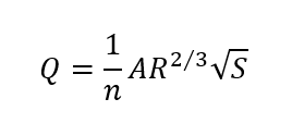
Where:
Q = flow rate
n = Manning’s roughness coefficient
A = cross-sectional area (having flow depth)
R = hydraulic radius
S = channel slope
For Steady State Peak Flow and Kinematic Wave routing methods, the channel slope (S) is interpreted as the conduit slope. In the case of Hydrodynamic routing, the channel slope (S) is interpreted as the friction slope.
However, for the user-defined Force Main conduits that are under pressurized flow, the user can either use the Hazen-Williams or Darcy-Weisbach equation.
Follow the steps below to select a flow routing method in GeoSTORM:
- From the Input ribbon menu, select the Scenario Manager command.
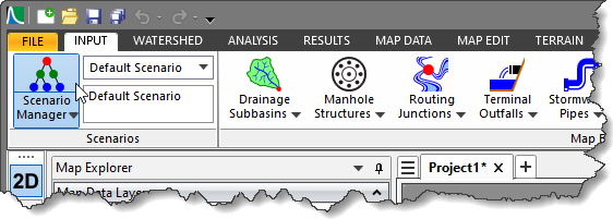
- The Scenario Manager dialog box will be displayed.

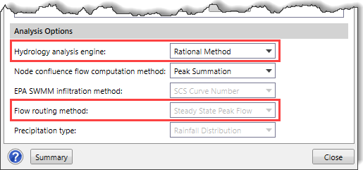
- Now, from the Flow routing method dropdown combo box, select the flow routing method to be used for routing the flow through the stormwater network.

- Note that the Flow routing method dropdown combo box will be displayed as disabled when the Rational Method is selected as the hydrology analysis engine.
The following sections explain the flow routing methods supported by GeoSTORM.
Hydrodynamic
The Hydrodynamic routing method allows the user to solve the complete one-dimensional Saint Venant flow equations and get the most theoretically accurate results. These equations consist of the continuity and momentum equations for conduits and the volume continuity equation at nodes.
This flow routing method makes it possible to represent pressurized flow when a closed conduit becomes full, such that flows can exceed the full normal flow value. Flooding occurs when the water depth at a node exceeds the maximum available depth, and the excess flow is either lost from the system or can pond atop the node and re-enter the drainage system.
The Hydrodynamic routing method can account for channel storage, backwater, entrance/exit losses, flow reversal, and pressurized flow. Since it couples together the solution for both water levels at nodes and flow in conduits, it can be applied to any general network layout, even those containing multiple downstream diversions and cyclic loops.
This flow routing method is preferred for systems subjected to significant backwater effects due to downstream flow restrictions and flow regulation via weirs and orifices. This generality comes at the price of having to use much smaller time steps, i.e., about thirty seconds or less (the software can automatically reduce the user-defined maximum time step as needed to maintain numerical stability).
Kinematic Wave
The Kinematic Wave routing method can solve the continuity equation along with a simplified form of the momentum equation in each conduit. The momentum equation assumes that the slope of the water surface equals the slope of the conduit.
The maximum flow that can be conveyed through a conduit is the full normal flow value. Any flow in excess of this entering the inlet node is either lost from the system or can pond atop the inlet node and be re-introduced into the conduit as capacity becomes available.
Kinematic Wave routing method allows flow and area to vary both spatially and temporally within a conduit. This can result in attenuated and delayed outflow hydrographs as inflow is routed through the channel.
However, the Kinematic Wave routing method cannot account for backwater effects, entrance/exit losses, flow reversal, or pressurized flow. Also, this flow routing method is restricted to dendritic network layouts. It can usually maintain numerical stability with moderately large time steps, i.e., about 1 to 5 minutes. If the limitations mentioned above are not expected to be significant, then this flow routing method can be an accurate and efficient alternative, especially for long-term simulations.
Steady State Peak Flow
The Steady State Peak Flow routing method represents the simplest type of routing possible (actually no routing) by assuming that within each computational time step flow is uniform and steady. Therefore, it simply translated inflow hydrographs at the upstream end of the conduit to the downstream end, with no delay or change in shape. This flow routing method uses the normal flow equation to relate flow rate to flow area (or depth).
The Steady State Peak Flow routing method cannot account for channel storage, backwater effects, entrance/exit losses, flow reversal, or pressurized flow. Also, this flow routing method can only be used with dendritic conveyance networks, where each node has only a single outflow link (unless the node is a flow divider, requiring two outflow links). This flow routing method is insensitive to the defined time step and is only suitable for preliminary analysis using long-term continuous simulations.
Notes:
- The Steady State Peak Flow and Kinematic Wave routing methods are not applicable to drainage systems forming a cyclic loop network (i.e., a directed flow path along a set of links that starts and ends at the same node). Refer to this article in our knowledge base to learn more about cyclic loop networks.
In such situations where cyclic loops exist in the drainage system, the Hydrodynamic routing method must be specified. - While using the Steady State Peak Flow or Kinematic Wave routing methods, the user must ensure that the conduit link (channel, pipe, or culvert) has a positive slope. In case of an adverse slope (i.e., negative slope), the Hydrodynamic routing method must be specified. Otherwise, the software will display an error while computing the analysis.