In GeoHECRAS software, the Unsteady Flow Data command allows the user to define the boundary conditions data necessary to perform an unsteady flow analysis. Unsteady flow data consists of external boundary conditions, internal boundary conditions, and global boundary conditions (Meteorological Data).
External boundary conditions are required to run an unsteady model. External boundary conditions must be established at all open ends (i.e., upstream and downstream ends) of each river reach (or 2D flow area) being modeled.
Internal boundary conditions are optional and allow the user to define gate operations and add flow within a river reach.
Global boundary conditions allow the user to define spatial precipitation and evapotranspiration data.
Follow the steps below to use the Unsteady Flow Data command:
- From the Input ribbon menu, select the Unsteady Flow Data command.

- The Unsteady Flow Data dialog box will be displayed.
The following sections describe how to use the Unsteady Flow Data command and interact with the above dialog box.
River Reach Data
This panel allows the user to define boundary conditions and initial flow and stage conditions data for performing the unsteady flow analysis. Note that the River Reach Data panel is used for 1D unsteady flow modeling.
The following subpanels are provided:
- Boundary Conditions
- Initial Flow & Stage Conditions
Boundary Conditions
This subpanel allows the user to define external and internal reach boundary conditions to be used in the unsteady flow analysis.
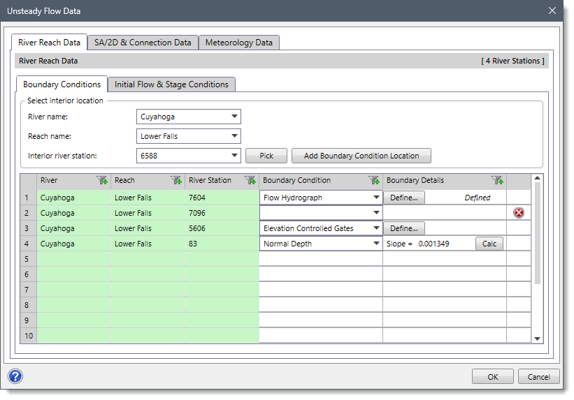
The Select interior location section allows the user to select the river, reach, and corresponding internal river cross section. Note that if a cross section has been preselected from the Map View before running this command, then the River name, Reach name, and Interior river station dropdown combo box fields will show the corresponding river, reach, and selected cross section.
Alternatively, the user can click the [Pick] button to manually select the cross section from the Map View. Clicking the [Pick] button causes the dialog box to temporarily disappear, and the user will be prompted to select an interior cross section from the Map View. Note that only one cross section can be selected at a time. After selecting a cross section, the dialog box will be redisplayed and the River name, Reach name, and Interior river station dropdown combo box fields will automatically update corresponding to the selected cross section. In addition, the selected cross section is highlighted on the Map View.
After selecting an interior cross section, the [Add Boundary Condition Location] button becomes enabled. Click the [Add Boundary Condition Location] button and a row will be added to the boundary conditions table defining the internal boundary condition location.
The Boundary Conditions subpanel contains a table that defines the boundary condition data. The software automatically lists the external boundary condition locations (most upstream and downstream cross sections) and inline/lateral structures in the table. The user is only required to enter the internal boundary condition locations. Note that the external boundary condition locations cannot be deleted from the table. However, the user can delete the interior boundary condition locations from the table.
To delete an interior boundary condition location from the table, click the [X] close button adjacent to the internal boundary condition row. The Remove Interior Location dialog box will be displayed.
Click the [Yes] button and the selected interior boundary condition location will be deleted from the table. To abort the process, click the [No] button.
The table in this subpanel contains the following data column entries:
- River
This read-only entry lists the river name.
- Reach
This read-only entry lists the reach name.
- River Station
This read-only entry lists the cross section river station.
- Boundary Condition
This dropdown combo box entry allows the user to select the type of boundary condition for each river station (cross section). The dropdown combo box provides the boundary condition types based upon the cross section location, as shown in the table below:
Boundary Condition Available for Locations Blank (empty entry, default) Normal Depth Downstream boundary Flow Hydrograph Downstream & upstream boundary Stage Hydrograph Downstream & upstream boundary Stage/Flow Hydrograph Downstream & upstream boundary Rating Curve Downstream boundary Lateral Inflow Hydrograph Interior cross section Uniform Lateral Inflow Interior cross section Interior Boundary Stage/Flow Interior cross section Groundwater Interflow Interior cross section Time Series Gate Opening Inline/Lateral structure Elevation Controlled Gates Inline/Lateral structure
- Boundary Details
This entry provides additional data for the selected boundary condition. This entry changes based upon the selected boundary condition type, as shown in the table below:
Boundary Condition Descriptions Empty Empty Normal Depth The user is required to enter the energy slope value. This value represents the energy grade slope at the downstream boundary. In addition, a [Calc] button is provided. If the energy slope is unknown, the user could approximate it by clicking the [Calc] button. Flow Hydrograph It can be used as either an upstream boundary or a downstream boundary condition. When this type of boundary condition is selected, a [Define…] button is provided. Clicking a [Define…] button will display a Flow Hydrograph dialog box to define the boundary condition data. Stage Hydrograph It can be used as either an upstream boundary or a downstream boundary condition. When this type of boundary condition is selected, a [Define…] button is provided. Clicking a [Define…] button will display a Stage Hydrograph dialog box to define the boundary condition data. Stage/Flow Hydrograph It can be used together as either an upstream or downstream boundary condition. When this type of boundary condition is selected, a [Define…] button is provided. Clicking a [Define…] button will display a Stage/Flow Hydrograph dialog box to define the boundary condition data. Rating Curve It can be used as a downstream boundary condition. When this type of boundary condition is selected, a [Define…] button is provided. Clicking a [Define…] button will display a Rating Curve dialog box to define the boundary condition data. Lateral Inflow Hydrograph It can be used as an internal boundary condition that allows the user to bring in flow at a specific point along the stream. When this type of boundary condition is selected, a [Define…] button is provided. Clicking a [Define…] button will display a Lateral Inflow Hydrograph dialog box to define the boundary condition data. Uniform Lateral Inflow Hydrograph It can be used as an internal boundary condition that allows the user to bring in a flow hydrograph and distribute it uniformly along the river reach between two user-specified cross section locations. When this type of boundary condition is selected, a [Define…] button is provided. Clicking a [Define…] button will display a Uniform Lateral Inflow Hydrograph dialog box to define the boundary condition data. Groundwater Interflow It is similar to a uniform lateral inflow in that the user enters an upstream and a downstream river station in which the flow passes back and forth. When this type of boundary condition is selected, a [Define…] button is provided. Clicking a [Define…] button will display a Groundwater Interflow dialog box to define the boundary condition data. Interior Boundary Stage/Flow It allows the user to enter a known stage hydrograph and/or a flow hydrograph, to be used as an internal boundary condition. When this type of boundary condition is selected, a [Define…] button is provided. Clicking a [Define…] button will display an Interior Boundary Stage/Flow dialog box to define the boundary condition data. Time Series Gate Openings It allows the user to enter a time series of gate openings for an inline gated spillway, a lateral gated spillway, or a gated spillway connecting two storage areas. When this type of boundary condition is selected, a [Define…] button is provided. Clicking a [Define…] button will display a Time Series Gate Openings dialog box to define the boundary condition data. Elevation Controlled Gates It allows the user to control when each gate will open and close as well as the opening and closing rates. When this type of boundary condition is selected, a [Define…] button is provided. Clicking a [Define…] button will display an Elevation Controlled Gates dialog box to define the boundary condition data.
Refer to this article in our knowledge base to learn more about boundary condition types
Initial Flow & Stage Conditions
This subpanel allows the user to define the initial flow and stage conditions for each reach to be used in the unsteady flow analysis. The user can establish the initial conditions of the system using either the Use Initial Conditions (Restart or Hotstart) File option or the Define Initial Flows option. To learn more about the Initial Flow & Stage Conditions subpanel, refer to this article in our knowledge base.
SA/2D & Connection Data
This panel allows the user to define storage area, 2D flow area, and SA/2D connection data for performing the unsteady flow analysis. Note that this panel is used for the storage area and 2D unsteady flow modeling.
The following subpanels are provided:
- SA/2D Flow Areas
- SA/2D BC Lines
- SA/2D Connection Gates
- Initial Stage Elevations
SA/2D Flow Areas
This subpanel provides a table in which the storage area and 2D flow area boundary conditions are defined.
The table in this subpanel contains the following data column entries:
- Storage Area/2D Flow Area
This read-only entry lists the IDs of the storage area and 2D flow area.
- Boundary Condition
This dropdown combo box entry allows the user to select the boundary condition types.
- Boundary Details
This entry provides additional data for the selected boundary condition. This entry changes based upon the selected boundary condition. Refer to the River Reach Data panel part of this article to learn more about the Boundary Details entry.
SA/2D BC Lines
This subpanel provides a table in which the 2D flow area boundary conditions lines are defined.
The table in this subpanel contains the following data column entries:
- Boundary Condition Line ID
This read-only entry lists the IDs of the 2D flow area boundary conditions lines.
- Boundary Condition
This dropdown combo box entry allows the user to select the boundary condition types.
- Boundary Details
This entry provides additional data for the selected boundary condition. This entry changes based upon the selected boundary condition. Refer to the River Reach Data panel part of this article to learn more about the Boundary Details entry.
SA/2D Connection Gates
This subpanel provides a table that lists the SA/2D connections in which the gates and outlet time series are defined.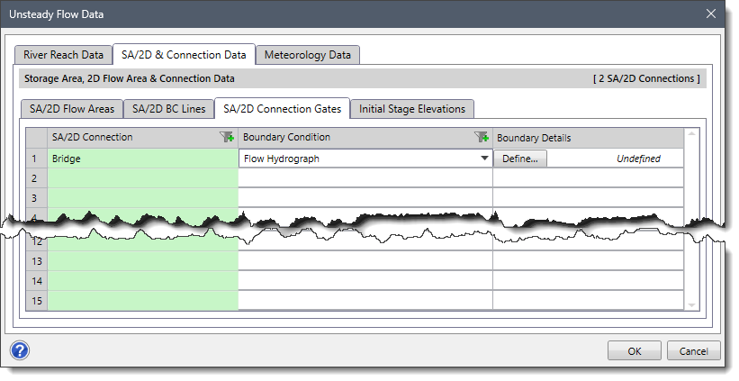
The table in this subpanel contains the following data column entries:
- SA/2D Connection
This read-only entry lists the IDs of the SA/2D connections.
- Boundary Condition
This dropdown combo box entry allows the user to select the boundary condition types.
- Boundary Details
This entry is adjacent to the Boundary Condition entry that provides additional data for the selected boundary condition. This entry changes based upon the selected boundary condition. Refer to the River Reach Data panel part of this article to learn more about the Boundary Details entry.
Initial Stage Elevations
This subpanel allows the user to define the initial stage elevations for storage areas and 2D flow areas defined in the model.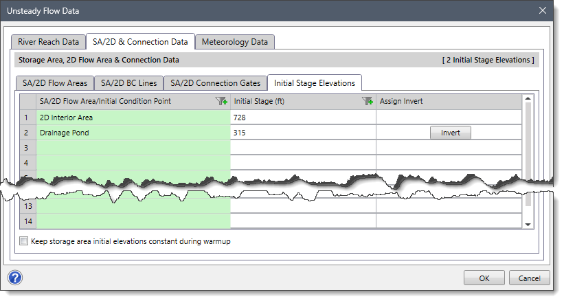
The table in this subpanel contains the following data column entries:
- SA/2D Flow Area/Initial Condition Point
This read-only entry lists the IDs of the storage area, 2D flow area, and initial condition point.
- Initial Stage
This entry can be left blank to simulate the area “starting dry.” Alternatively, the user can start with a constant water surface elevation by entering an elevation value for each storage area and 2D flow area. By default, the software will use the initial stage of the storage area and 2D flow area.
- Assign Invert
This entry allows the user to overwrite the stage elevation of the storage area with the invert elevation in the Initial Stage column by clicking the [Invert] button.
- Keep storage area initial elevations constant during warmup
This checkbox option allows the software to keep water surface levels in storage areas at the user-entered value during the warmup period (e.g., a dry storage area will still be dry at the end of the warmup even if it had incoming flow). If a warmup period is not used, then this checkbox option will have no effect. Refer to this article in our knowledge base to learn how to perform a warmup run.
Meteorology Data
This panel allows the user to utilize meteorology (i.e., precipitation and evapotranspiration) data for unsteady flow modeling.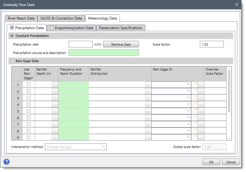
The following subpanels are provided:
- Precipitation Data
- Evapotranspiration Data
- Rasterization Specifications
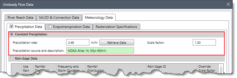
Precipitation Data
This subpanel allows the user to define the spatial precipitation data for unsteady flow modeling. By default, the checkbox at this subpanel is unchecked and contents are disabled (i.e., grayed out). Check the checkbox at the Precipitation Data subpanel to enable the contents of this subpanel.
The following sections are provided in this subpanel:
- Constant Precipitation
- Rain Gage Data
Constant Precipitation
This section allows the user to define the constant precipitation rate and scale factor for the precipitation rate.
The following options are provided:
- Precipitation rate
This entry field defines the constant precipitation rate. Click the [Retrieve Data] button to retrieve the precipitation data. On clicking the [Retrieve Data] button, the Unsteady Flow Data dialog box will temporarily disappear, and the Lookup Rainfall Intensity dialog box will be displayed.
In the above dialog box, the user can select the location from which the rainfall intensity data are to be retrieved. Once the desired location is selected, click the Precipitation data source dropdown combo box to select the precipitation data sources that are available. After selecting the precipitation data source, click the [Retrieve] button to retrieve the rainfall intensity data for the selected location.
Upon successful retrieval of the rainfall intensity data, the software populates the data in the table provided under the Rainfall intensity subsection. This table displays the rainfall intensity values for various storm frequencies and durations. Select the required rainfall intensity rate, then click the [OK] button. The Unsteady Flow Data dialog box will be redisplayed, and the selected rainfall intensity rate will be displayed in the Precipitation rate entry. Refer to this article in our knowledge base to learn more about how to retrieve rainfall intensity data.
- Scale factor
This entry field defines the scale factor that will adjust the defined rain gage data. By default, the software uses a default value of 1.00.
- Precipitation source and description
This read-only field displays the reference information of the precipitation data retrieved (i.e., precipitation data source, storm frequency and duration, etc.).
Rain Gage Data
This section allows the user to define the precipitation data that varies with time using a rain gage and then interpolates over the model area using a raster grid. Select the Rain Gage Data radio button option to enable this section. Otherwise, this section is disabled (i.e., grayed out).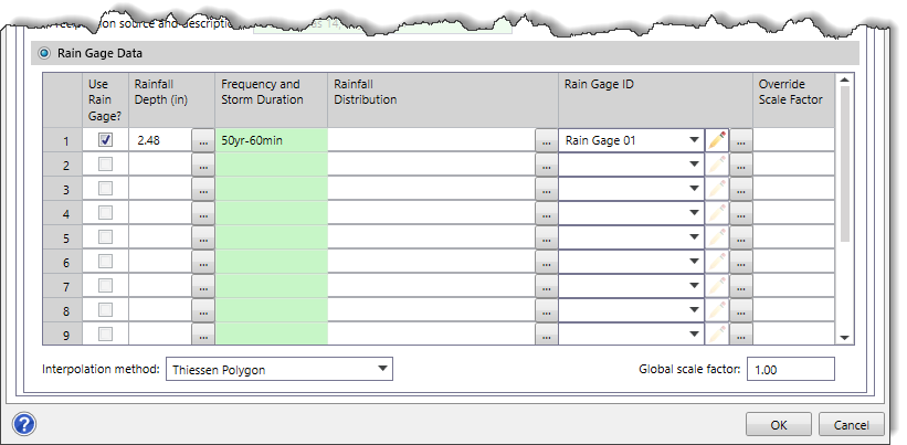
The table in this section contains the following data column entries:
- Use Rain Gage?
This checkbox entry allows the user to specify whether to use the defined rain gage. The checkboxes allow the user to turn on or off various rain gages to experiment with the effect of different rain gages being included in the simulation. By default, this entry is unchecked.
- Rainfall Depth
This entry allows the user to specify the total rainfall depth for the defined rain gage. Click the […] button to retrieve the rainfall depth to be assigned to the defined rain gage. On clicking the […] button, the Unsteady Flow Data dialog box will temporarily disappear, and the Lookup Rainfall Depth dialog box will be displayed. This dialog box allows the user to select the rainfall depth. After selecting the rainfall depth, the Unsteady Flow Data dialog box will be redisplayed, and the selected rainfall depth will be displayed in the Rainfall Depth entry. Refer to this article in our knowledge base to learn more about how to retrieve rainfall depth.
- Frequency and Storm Duration
This read-only entry displays the reference information of the rainfall data retrieved (i.e., frequency (years) and storm duration).
- Rainfall Distribution
This entry allows the user to select the rainfall distribution to be used for creating a rain gage. Click the […] button to select the rainfall distribution to be applied for creating rain gage. On clicking the […] button, the Unsteady Flow Data dialog box will temporarily disappear, and the Rainfall Distribution dialog box will be displayed. This dialog box allows the user to retrieve the rainfall distribution. After selecting the rainfall distribution, the Unsteady Flow Data dialog box will be redisplayed, and the selected rainfall distribution will be displayed in the Rainfall Distribution entry. Refer to this article in our knowledge base to learn more about how to retrieve rainfall distribution.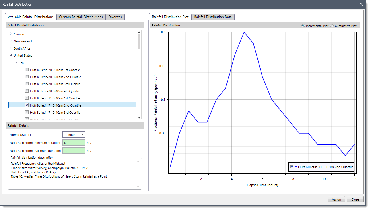
- Rain Gage ID
This dropdown combo box entry lists all the rain gages that are defined in the current scenario. The edit option (i.e., pencil icon) allows the user to edit the rain gage ID. Click the […] button to define rain gage point locations and corresponding precipitation data. On clicking the […] button, the Unsteady Flow Data dialog box will temporarily disappear, and the Rain Gage Data dialog box will be displayed. This dialog box allows the user to define the rain gage data. After defining the rain gage data, the Unsteady Flow Data dialog box will be redisplayed, and the defined rain gage will be listed in the Rain Gage ID dropdown combo box entry. Refer to this article in our knowledge base to learn more about how to define rain gage time series data.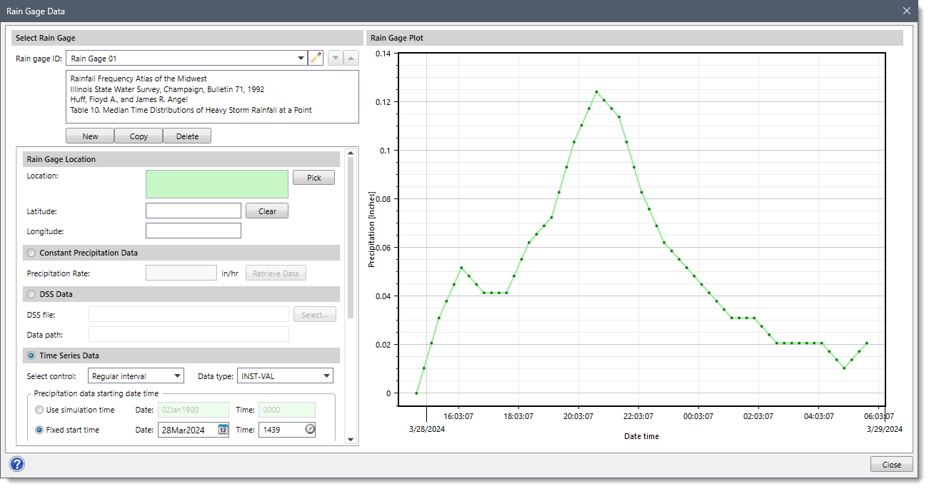
- Override Scale Factor
This entry contains an optional scale factor that will adjust the defined rain gage data. This scale factor will override the defined value of the Global scale factor entry for an individual rain gage.In addition, the following additional options are provided in this section:
- Interpolation method
This dropdown combo box allows the user to select the interpolation method that defines how the rain gage data will be interpolated across the 2D precipitation grid. The following interpolation methods are available: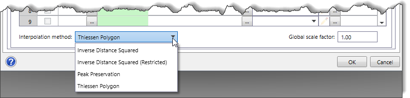
- Inverse Distance Squared
This interpolation method computes a weighted rainfall depth for each rainfall time-step individually by using the inverse square of the distance weighting method to all rain gages near a specific 2D precipitation cell. If the defined rainfall data have an hourly time-step, then the inverse square of the distance weighting method is applied individually at each one-hour time-step. - Inverse Distance Squared (Restricted)
This interpolation method works similarly to the Inverse Distance Squared method but with an additional step. Initially, it triangulates all rain gages. Then, when a 2D precipitation cell lies inside of a specific triangle, only the three gages that form the triangle are used in the storm weighting process. This method prevents rain gages that are far away from a 2D precipitation cell from being used and limits the interpolation to the three closest rain gages to each 2D precipitation cell. - Peak Preservation
This interpolation method tries to retain rainfall intensities within a storm as it moves across a watershed. The Inverse Distance Squared and Inverse Distance Squared Restricted methods have the problem of diminishing the rainfall intensities when the rainfall timing is different at each rain gage being used for the interpolation. In such cases, the Peak Preservation method can be utilized. The Peak Preservation method takes all the rain gages being used for a particular 2D precipitation cell and finds the center of mass of the precipitation for each of the rain gages. Next, all gaged data is lined up by the center of mass. Then the data are interpolated on a time-step by time-step basis. Finally, the interpolated data are shifted back to the correct time to account for the location of the 2D precipitation cell between the rain gages. - Thiessen Polygon
This interpolation method is a traditional method often used in hydrologic modeling. This method draws a line between two rain gages and finds the half distance between each rain gage. This distance calculation process is repeated for all rain gages. Polygons are then formed by the linear bisection lines between the rain gages. The software does this to figure out which rain gage should be used to determine the rainfall event pattern. For 2D precipitation cells that are closest to a rain gage (i.e., inside that rain gage’s Thiessen polygon), the rain gage will be used to define the rainfall pattern (intensity versus time). However, the storm total rainfall applied to each 2D precipitation cell is computed using the Inverse Distance Squared method to determine a weighted storm total rainfall for each 2D precipitation cell. The storm total rainfall is then applied to the previously determined nearest rain gage’s rainfall event pattern to define the rainfall distribution for that specific 2D precipitation cell.
- Inverse Distance Squared
- Global scale factor
This entry field defines the scale factor that will adjust all defined rain gage data. However, this scale factor can be overridden at an individual rain gage from the Override Scale Factor column entry.
Evapotranspiration Data
This subpanel allows the user to define the evapotranspiration data for unsteady flow modeling. By default, the checkbox at this subpanel is unchecked and contents are disabled (i.e., grayed out). Check the checkbox at the Evapotranspiration Data subpanel to enable the contents of this subpanel.
The following sections are provided in this subpanel:
- Constant Evapotranspiration
- Evapotranspiration Gage Data
Constant Evapotranspiration
This section allows the user to define the constant evapotranspiration rate and scale factor for the evapotranspiration rate.
The following options are provided:
- Evapotranspiration rate
This entry field defines the constant evapotranspiration rate.
- Scale factor
This entry field defines the scale factor that will adjust the defined evapotranspiration gage data. By default, the software uses a default scale factor of 1.00.
Evapotranspiration Gage Data
This section allows the user to define the evapotranspiration data that vary with time using an evapotranspiration gage and then interpolated over the model area using a raster grid. Select the Evapotranspiration Gage Data radio button option to enable this section. Otherwise, this section is disabled (i.e., grayed out).
The table in this section contains the following data column entries:
- Use Evapotranspiration Gage?
This checkbox entry allows the user to specify whether to use the defined evapotranspiration gage. The checkboxes allow the user to turn on or off various evapotranspiration gages to experiment with the effect of different evapotranspiration gages being included in the simulation. By default, this entry will be unchecked.
- Evapotranspiration Gage ID
This dropdown combo box entry lists all the evapotranspiration gages that are defined in the current scenario. The edit option (i.e., pencil icon) allows the user to edit the evapotranspiration gage ID. Click the […] button to define evapotranspiration gage point locations and corresponding precipitation data. On clicking the […] button, the Unsteady Flow Data dialog box will temporarily disappear, and the Evapotranspiration Gage Data dialog box will be displayed. This dialog box allows the user to select the evapotranspiration gage data. After selecting the evapotranspiration gage data, the Unsteady Flow Data dialog box will be redisplayed, and the selected evapotranspiration gage will be listed in the Evapotranspiration Gage ID dropdown combo box entry. Refer to this article in our knowledge base to learn more about how to define evaporation gage time series data.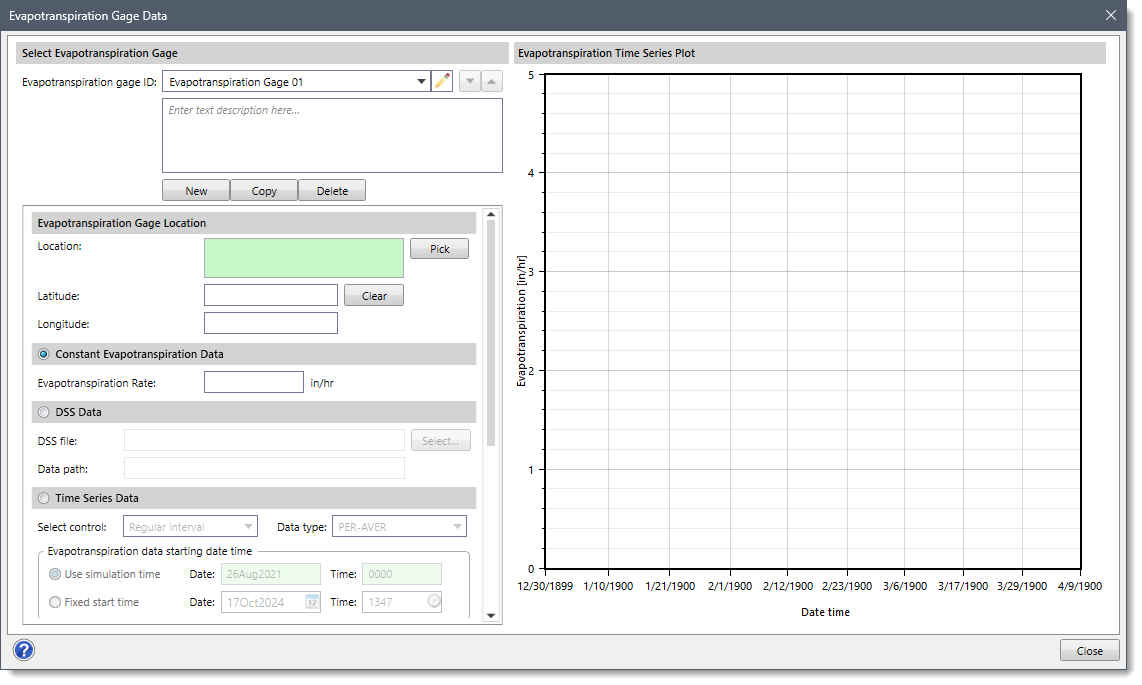
- Summary
This entry defines additional information to describe the selected evapotranspiration gage.
- Override Scale Factor
This entry contains an optional scale factor that will adjust the defined evapotranspiration gage data. This scale factor will override the defined value of the Global scale factor entry for an individual evapotranspiration gage.In addition, the following additional options are provided in this section:
- Interpolation method
This dropdown combo box allows the user to select the interpolation method that defines how the evapotranspiration gage data will be interpolated across the 2D precipitation grid. The following interpolation methods are available:
- Inverse Distance Squared
This interpolation method computes a weighted depth of rainfall for each time period individually by using the inverse square of the distance weighting method for all of the gages near a specific cell. If the rainfall data are hourly, then the inverse square of the distance weighting method is done individually for each one-hour time step. - Inverse Distance Squared (Restricted)
This interpolation method does the same thing as the Inverse Distance Squared method, except it first triangulates all the gages. Then, if a cell lies inside of a specific triangle, only the three gages that form the triangle are used in the storm weighting process. This method prevents gages that are far away from being used and limits the interpolation to the three closest gages to the cell. - Nearest Neighbor
This interpolation method uses a simple approach to interpolate cell values. Rather than computing a weighted depth or triangulating the gage network, it just finds out the nearest neighboring cell with a known value and assumes the same value to its neighboring cell, thereby interpolating the whole rain gage domain.
- Inverse Distance Squared
- Global scale factor
This entry field defines the scale factor that will adjust all defined evapotranspiration gage data. However, this scale factor can be overridden at an individual evapotranspiration gage from the Override Scale Factor column entry
Rasterization Specifications
This subpanel allows the user to define the extents (or limits) for how the point gage data will be rasterized. This extent will depend on the location of the HEC-RAS model, rain gages, and/or the evapotranspiration gages created.
Defining Raster Extents
The Define Raster Extents section allows the user to define the extent of the raster file to be generated.
The following radio button options are provided:
- HEC-RAS model and gage extents
This option causes the raster to be equal to the extent of the HEC-RAS model and defined gages, plus a 1,000 ft (300 meters) buffer outside these limits. By default, this option is selected.
- Gage extents
This option causes the raster to be equal to the extent of the defined gages, plus a 1,000 ft (300 meter) buffer outside these limits.
- User-defined limits
This option allows the user to manually define the raster limits from Map View. After selecting this option, the user can click the [Pick] button to draw a rectangular region on the Map View that will define the meteorology raster grid limits.
Defining Grid Resolution
The Define Grid Resolution section allows the user to define the coordinate extents for how the point gage data will be rasterized.
The following options are provided:
- Number of columns
This read-only field displays the number of columns contained in the raster grid.
- Number of rows
This read-only field displays the number of rows contained in the raster grid.
- Total number of cells
This read-only field displays the total number of cells contained in the defined raster grid.
- Raster cell size
This entry field is used to manually define the size of raster grid cells. The finer the grid resolution (or smaller the cell size) defined, the greater the detail that can be represented in the generated raster grid. Note that if the user changes the raster cell size value, the software will automatically recompute the number of columns, rows, and total number of cells based on the defined raster extents. By default, the software uses a default value of 1000 ft (300 meters).
Defining Data Extrapolation Methods
The Define Data Extrapolation Methods section allows the user to define the extrapolation methods of the defined rain gage (or evapotranspiration gage) data to the 2D meteorology grid.
The following options are provided:
- TIN extrapolation method
This dropdown combo box allows the user to select the extrapolation method used to generate the precipitation map. The following extrapolation methods are provided:
- None
If this option is selected, no extrapolation will be used to generate the precipitation map. - Nearest Segment
This extrapolation method extends the Triangulated Irregular Network (TIN) beyond its original data points to estimate surface values in areas without data. This method involves identifying the two nearest TIN segments to each extrapolation point and calculating weights based on their distances. These weights are used to interpolate the surface value at the extrapolation point, considering the linear variation within the TIN triangle. This process is repeated for all extrapolation points in the defined area. While this method provides a straightforward approach, its accuracy may be limited when dealing with highly irregular or complex data. - Nearest Triangle
This extrapolation method is used for Triangular Irregular Network(TIN) extrapolation. This method estimates values outside the known data points by finding the nearest triangle in the TIN containing the target point and assuming a smooth variation within that triangle. The method involves identifying the target point, finding the nearest triangle, calculating barycentric coordinates, interpolating the value using the weights of the triangle vertices, and considering the interpolated value as an estimate for the target point. However, it has limitations in modeling complex or non-linear surfaces and carries inherent uncertainty in extrapolated results.
- None
- Resampling method
This dropdown combo box allows the user to select the resampling method used to create the precipitation map. The following resampling methods are provided.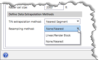
- None/Nearest
This resampling method is used to convert point data into raster format. It can be used to assign a single value to each raster cell based on the nearest data point without considering attributes using the nearest neighbor algorithm. This method is suitable when attribute information is not required or when it does not need to be preserved. - Linear/Render Block
This resampling method involves dividing the area into smaller blocks, performing linear interpolation within each block to estimate values, rendering the estimated values onto a grid, and resampling the grid, if necessary, to a different resolution.
- None/Nearest