Subbasin Data – Selecting an Infiltration Method -CivilGEO Knowledge Base

Subbasins define the drainage area polygons that produce runoff to the other elements in the model. While a subbasin element conceptually represents infiltration, surface runoff, and subsurface processes interacting together, the actual infiltration loss calculations are performed by an infiltration method contained within the subbasin.

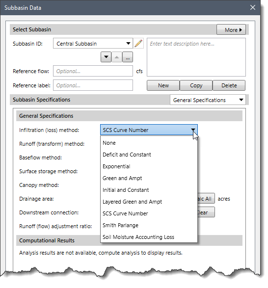
There are many different infiltration methods provided with HEC-HMS. Some of the methods are designed primarily for simulating events, while others are intended for continuous simulation. All of the methods conserve mass. That is, the sum of infiltration and precipitation left on the surface will always be equal to total incoming precipitation.

The table below shows the various methods’ suitability for an event and continuous simulation.

Infiltration (Loss) Method	Event	Continuous
Deficit and constant		Yes
Exponential	Yes
Green and Ampt	Yes
Initial and constant	Yes
Layered Green and Ampt		Yes
SCS curve number	Yes
Smith Parlange	Yes
Soil moisture accounting		Yes

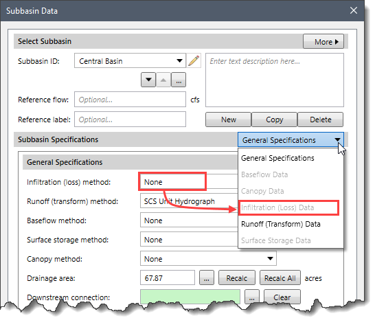
In GeoHECHMS, the infiltration method for a subbasin can be selected from the General Specifications section of the Subbasin Data dialog box.

Follow the steps given below to select an infiltration method:

From the Input ribbon menu, select the Subbasin Data command.
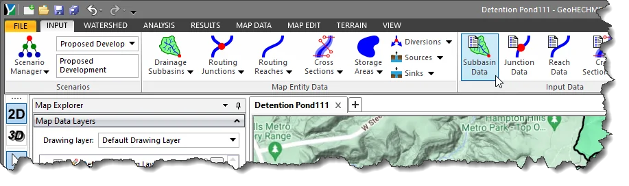
The Subbasin Data dialog box will be displayed.
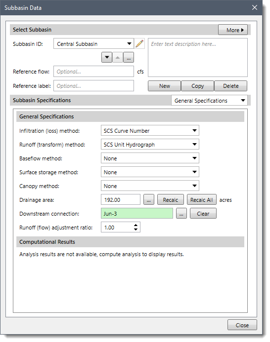
From the Subbasin ID dropdown combo box, select the subbasin to assign an infiltration method.
From the Infiltration (loss) method dropdown combo box, select the infiltration method.
To enter the data for the selected infiltration method, select the Infiltration (Loss) Data option from the Subbasin Specifications dropdown combo box.
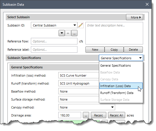
The Infiltration (Loss) Data panel will be displayed. Note that the Infiltration (Loss) Data panel content changes based upon the infiltration (loss) method selected in the General Specifications section.

The following sections describe the different infiltration methods and how to define the data for each method in the Infiltration (Loss) Data panel.

Infiltration Method: None

When None is selected for the Infiltration (Loss) Method, then the Infiltration (Loss) Data dropdown combo box entry is disabled (i.e., grayed out).
Selecting None as infiltration method

Infiltration Method: Deficit and Constant

The deficit and constant infiltration method uses a single soil layer to account for continuous changes in moisture content. This method is used for continuous simulation.

It should be combined with a canopy method that will extract water from the soil in response to potential evapotranspiration computed in the meteorologic model. The soil layer will dry out as the canopy extracts soil water between precipitation events. There will be no soil water extraction unless a canopy method is selected. To learn how to select a canopy method for a subbasin, refer to this article in our knowledge base.

It may also be combined with a surface storage method that will hold water on the land surface. The water in surface storage infiltrates the soil layer. The infiltration rate is determined by the capacity of the soil layer to accept water. To learn how to select a surface storage method for a subbasin, refer to this article in our knowledge base.

When Deficit and Constant is selected for the Infiltration (Loss) Method, the following data panel will be displayed.
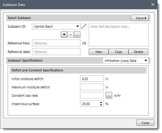
Infiltration (Loss) Data panel for Deficit and Constant method

The following input parameters are provided in the data panel:

Initial moisture deficit
This entry field defines the initial condition for the method. At the start of the simulation, it is the amount of water required to fill the soil layer to the maximum storage.
Maximum moisture deficit
This entry field is used to specify the total amount of water the soil layer can hold as an effective depth.
Constant loss rate
This entry field defines the infiltration and percolation rates when the soil layer is saturated. Clicking on the […] lookup button will display a Soil Saturated Hydraulic Conductivity lookup table dialog box.
Impervious surface
The field defines the percentage of the subbasin area that is impervious. No loss calculations are carried out on the impervious area. All precipitation on that portion of the subbasin becomes excess precipitation subject to surface storage and direct runoff. Note that the user can automatically compute the percent imperviousness for each subbasin using Compute % Impervious command. Refer to this article in our knowledge base to learn more about this command.

Infiltration Method: Exponential

The exponential infiltration method is empirical and should not be used without calibration. This method should only be used for event simulation. It represents incremental infiltration as an exponentially decreasing function of accumulated infiltration. It includes the option for increased initial infiltration when the soil is particularly dry before the arrival of a storm. Before using this method, consideration should be given to the Green and Ampt method (explained below) because it produces a similar exponential decrease in infiltration and uses parameters with better physical interpretation.

When Exponential is selected for the Infiltration (Loss) Method, the following data panel will be displayed.
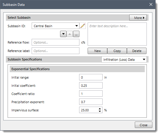
Infiltration (Loss) Data panel for Exponential method

The following input parameters are provided in the data panel:

Initial range
This entry field specifies the amount of initially accumulated infiltration during which the loss rate increases. This parameter is a function of antecedent soil moisture deficiency and is usually storm-dependent.
Initial coefficient
This entry field specifies the starting loss rate coefficient on the exponential infiltration curve. It is assumed to be a function of infiltration characteristics and consequently may be correlated with soil type, land use, vegetation cover, and other properties of a subbasin.
Coefficient ratio
This entry field specifies the rate at which the exponential decrease in infiltration capability proceeds. It may be considered a function of the ability of the surface of a subbasin to absorb precipitation and should be reasonably constant for large, homogeneous areas.
Precipitation exponent
This entry field defines the influence of precipitation rate on subbasin-average loss characteristics. It reflects the manner in which storms occur within an area and may be considered a characteristic of a particular region. It varies from 0.0 up to 1.0.
Impervious surface
The field defines the percentage of the subbasin area that is impervious.

Infiltration Method: Green and Ampt

The Green and Ampt infiltration method is essentially a simplification of the comprehensive Richard’s equation for unsteady water flow in soil. This method should only be used for event simulation and not for a continuous simulation where there is an extended dry period(s) between precipitation events. It assumes the soil is initially at uniform moisture content, and infiltration occurs with so-called piston displacement. It is also assumed that the soil layer is infinitely deep, so reaching saturation can be defined purely by the Green and Ampt equation. The method automatically accounts for ponding at the soil-air interface.

When Green and Ampt is selected for the Infiltration (Loss) Method, the following data panel will be displayed.
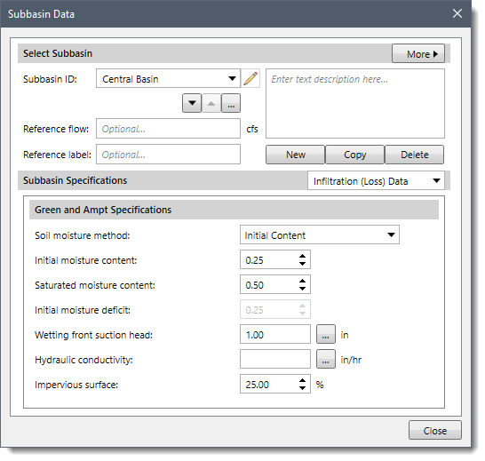
Infiltration (Loss) Data panel for Green and Ampt method

The following input parameters are provided in the data panel:

Soil moisture method
This dropdown combo box allows the user to select a method for specifying the initial soil moisture state. Two available options are Initial Content and Initial Deficit.
Initial moisture content
This entry field allows the user to specify the initial soil moisture state in terms of moisture content. Note that this field is only available when Initial Content is selected for the Soil moisture method. Otherwise, this entry is unavailable (i.e., grayed out).
Saturated moisture content
This entry field specifies the maximum water holding capacity in terms of volume ratio. It is often assumed to be the total porosity of the soil. Note that this field is only available when Initial Content is selected for the Soil moisture method. Otherwise, this entry is unavailable (i.e., grayed out).
Initial moisture deficit
This entry field allows the user to specify the initial soil moisture state in terms of a deficit. Note that this field is only available when Initial Deficit is selected for the Soil moisture method. Otherwise, this entry is unavailable (i.e., grayed out).
Wetting front suction head
This entry field is used to specify the wetting front suction. It is generally assumed to be a function of the soil texture. Clicking on the […] lookup button will display a Soil Suction lookup table dialog box.
Hydraulic conductivity
This entry field is used to specify the hydraulic conductivity. It can be estimated from field tests or approximated by knowing the soil texture. Clicking on the […] lookup button will display a Soil Saturated Hydraulic Conductivity lookup table dialog box.
Impervious surface
The field defines the percentage of the subbasin area that is impervious.

Infiltration Method: Initial and Constant

The initial and constant infiltration method is very simple but appropriate for watersheds lacking detailed soil information. It is also suitable for certain types of flow-frequency studies. This method should only be used for event simulation.

When Initial and Constant is selected for the Infiltration (Loss) Method, the following data panel will be displayed.
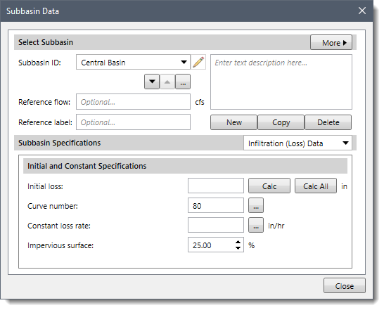
Infiltration (Loss) Data panel for Initial and Constant method

The following input parameters are provided in the data panel:

Initial loss
This entry field specifies the amount of incoming precipitation infiltrated or stored in the watershed before surface runoff begins. There is no recovery of the initial loss during periods without precipitation. Clicking the [Calc] button will cause the software to automatically compute the initial loss for the selected subbasin. Click the [Calc All] to compute the initial loss for all the subbasins.
Curve number
This entry field defines the curve number for the subbasin used to determine how much runoff occurs based upon the Land Use (or Land Cover) and the underlying Hydrologic Soil Type. Note that the user can automatically compute the curve number for each subbasin using Compute CN command. Refer to this article in our knowledge base to learn more about this command. Clicking the […] lookup button will display the SCS Curve Number lookup table dialog box.
Constant loss rate
This entry field specifies the rate of infiltration that will occur after the initial loss is satisfied. The same rate is applied regardless of the length of the simulation.
Impervious surface
The field defines the percentage of the subbasin area that is impervious.

Infiltration Method: Layered Green and Ampt

The layered Green and Ampt infiltration method uses two soil layers (layer 1 and layer 2) to account for continuous changes in moisture content. This method is based on algorithms originally developed for the Guelph Agricultural Watershed Storm-Event Runoff (GAWSER) model. This method should only be used for continuous simulation.

Two soil layers are used to represent the dynamics of water movement in the soil. Surface water infiltrates into the upper layer, called layer 1. Layer 1 produces seepage to the lower layer, called layer 2. Both layers are functionally identical but may have separate and distinct parameters. Separate parameters can be used to represent layered soil profiles and allow for a better representation of stratified soil drying between storms. Each layer is described using bulk depth and water content values for saturation, field capacity, and wilting point. Soil water in layer 2 can percolate out of the soil profile.

This method is intended to be used in combination with the linear reservoir baseflow method. When used in this manner, the percolated water can be split between baseflow and aquifer recharge. Refer to this article in our knowledge base to learn how to select a baseflow method for a subbasin.

This method can also be used in combination with a canopy method and surface storage method.

When Layered Green and Ampt is selected for the Infiltration (Loss) Method, the following data panel will be displayed.
Infiltration (Loss) Data panel for Layered Green and Ampt method

The following input parameters are provided in the data panel:

Layer 1 / Layer 2 initial moisture content
These entry fields are used to set the amount of soil water at the beginning of a simulation for the two soil layers. The values should be specified in terms of volume ratio.
Hydraulic conductivity
This entry field is used to specify the hydraulic conductivity. It can be estimated from field tests or approximated by knowing the surface soil texture. Clicking on the […] lookup button will display a Soil Saturated Hydraulic Conductivity lookup table dialog box.
Max seepage
This entry field is used to specify the maximum seepage at the bottom of layer 1. Field tests or the soil texture at the bottom of layer 1 can be used to estimate this value.
Max percolation
This entry field is used to specify the maximum percolation at the bottom of layer 2. Field tests or the soil texture at the bottom of layer 2 can be used to estimate this value.
Wetting front suction head
This entry field is used to specify the wetting front suction. It is generally assumed to be a function of the soil texture. Clicking on the […] lookup button will display a Soil Suction lookup table dialog box.
Dry duration
This entry field is used to set the amount of time that must pass after a storm event to recalculate the initial condition for the Green and Ampt equation. It has been found that 12 hours often works well.
Impervious surface
The field defines the percentage of the subbasin area that is impervious.
Layer 1 thickness
This entry field defines the bulk depth of soil measured from the ground surface down to the bottom of layer 1.
Layer 2 thickness
This entry field defines the bulk depth of soil measured from the bottom of layer 1 down to the bottom of layer 2.
Layer 1/ Layer 2 saturated moisture content
These entry fields are used to specify the maximum water holding capacity in terms of volume ratio for the two soil layers. These values define the total porosity of the soil.
Layer 1 / Layer 2 field capacity
These entry fields specify the point where the soil naturally stops seeping under gravity. The values should be specified in terms of volume ratio.
Layer 1 / Layer 2 wilting point
These entry fields specify the amount of water remaining in the soil layers when plants are no longer capable of extracting it. The values should be specified in terms of volume ratio.

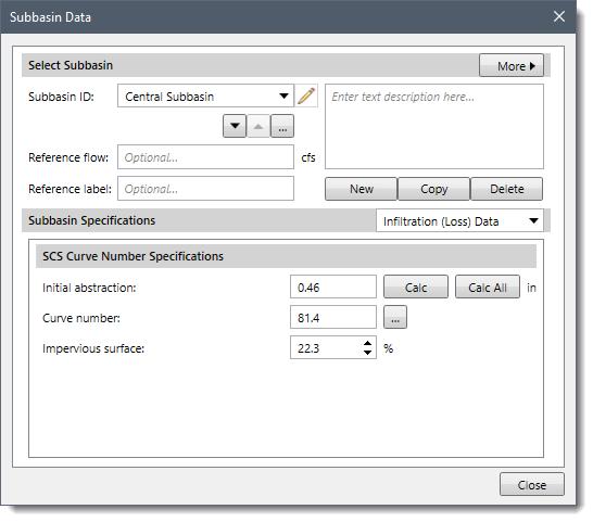
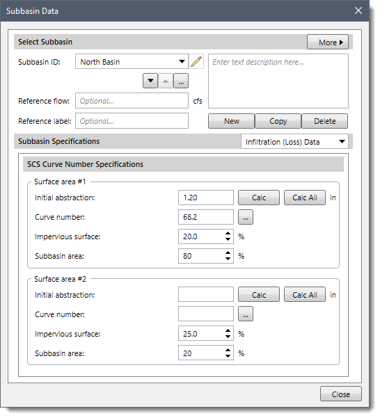
Infiltration Method: SCS Curve Number

The Soil Conservation Service (SCS) curve number method implements the curve number methodology for incremental losses (NRCS, 2007). The SCS curve number loss method should only be used for event simulation. Originally, the methodology was intended to calculate total infiltration during a storm. The software computes incremental precipitation during a storm by recalculating the infiltration volume at the end of each time interval. Infiltration during each time interval is the difference in volume at the end of two adjacent time intervals.

When SCS Curve Number is selected for the Infiltration (Loss) Method, the following data panel will be displayed.
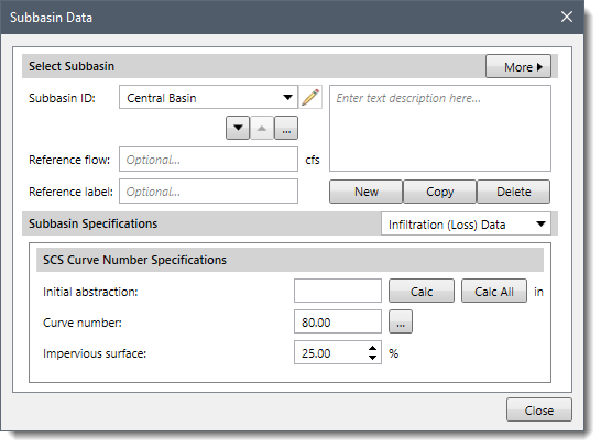
Infiltration (Loss) Data panel for SCS Curve Number method

The following input parameters are provided in the data panel:

Initial abstraction
This entry field allows the user to enter an initial abstraction. The initial abstraction defines the amount of precipitation that must fall before surface excess results. However, it is not the same as an initial interception or loss since changing the initial abstraction changes the infiltration response later in the storm. If this field is left blank, it will be automatically calculated as 0.2 times the potential retention, which is calculated from the curve number.
Curve number
This entry field allows the user to enter a curve number.
Impervious surface
The field defines the percentage of the subbasin area that is impervious.

Infiltration Method: Smith Parlange

The Smith Parlange infiltration method approximates Richard’s equation for infiltration into the soil. It assumes that the wetting front can be represented with an exponential scaling of the saturated conductivity. This linearization approach allows the infiltration computations to proceed quickly while maintaining a reasonable approximation of the wetting front. This method should only be used for event simulation.

When Smith Parlange is selected for the Infiltration (Loss) Method, the following data panel will be displayed.
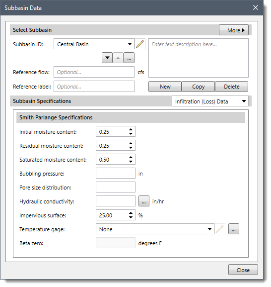
Infiltration (Loss) Data panel for Smith Parlange method

The following input parameters are provided in the data panel:

Initial moisture content
This field specifies the initial saturation of the soil at the beginning of a simulation. It should be specified in terms of volume ratio.
Residual moisture content
This field specifies the amount of water remaining in the soil after all drainage has ceased. It should be specified in terms of volume ratio.
Saturated moisture content
This field specifies the maximum water holding capacity in terms of volume ratio. It is often assumed to be the total porosity of the soil.
Bubbling pressure
This entry field specifies the bubbling pressure, also known as the wetting front suction. It is generally assumed to be a function of the soil texture.
Pore size distribution
This entry field specifies how the total pore space is distributed in different size classes. It is typically assumed to be a function of soil texture.
Hydraulic conductivity
The entry field specifies the hydraulic conductivity as the effective saturated conductivity. It can be estimated from field tests or approximated by knowing the soil texture.
Impervious surface
The field defines the percentage of the subbasin area that is impervious.
Temperature gage
This dropdown combo box lists temperature gage time series. The temperature gage is used to adjust for water density, water viscosity, and matric potential versus temperature. If no temperature gage is defined, then a temperature of 25° C (or 75° F) is assumed. The temperature gage must be defined in the Temperature Gage Data dialog box before selecting it.

Clicking the […] button will display the Temperature Gage Data dialog box, which allows the user to define temperature gages.

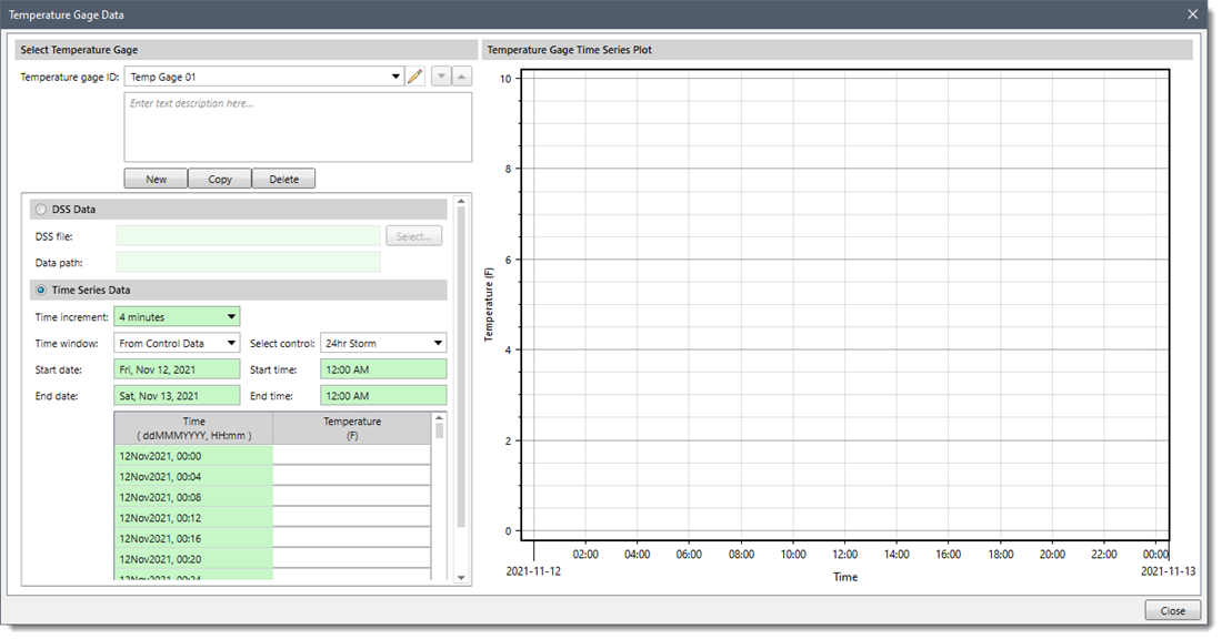The user may enter the time-series values by manually typing them or using the clipboard to copy and paste. Alternatively, the user may load the time-series data from a HEC-DSS file.
Beta zero
This entry field is used to define the beta zero parameter. This parameter is used to correct the matric potential based on temperature, which is generally a function of soil texture.

Infiltration Method: Soil Moisture Accounting Loss

The soil moisture accounting loss method uses three soil layers to account for continuous changes in moisture content throughout the vertical profile of the soil. This method is intended to be used for continuous simulation. This method can also be used in combination with a canopy and surface storage method.

Three soil layers are used in this method to represent the dynamics of water movement in the soil. Layers include soil storage, upper groundwater, and lower groundwater. The groundwater layer is not designed to represent aquifer processes. It is intended to be used for representing shallow inter-flow processes. The soil layer is subdivided into an upper zone and a tension zone. Soil water only percolates from the upper zone while water in the tension zone resists percolation. Water in the upper groundwater layer percolates to the lower groundwater layer.

The soil moisture accounting loss method is designed to be used in combination with the linear reservoir baseflow method. When used in this way, water can move laterally out of upper and lower groundwater layers to enter baseflow. Water percolating out of the lower groundwater layer can be split between entering baseflow and leaving the land surface as aquifer recharge.

When Soil Moisture Accounting Loss is selected for the Infiltration (Loss) Method, the following data panel will be displayed.
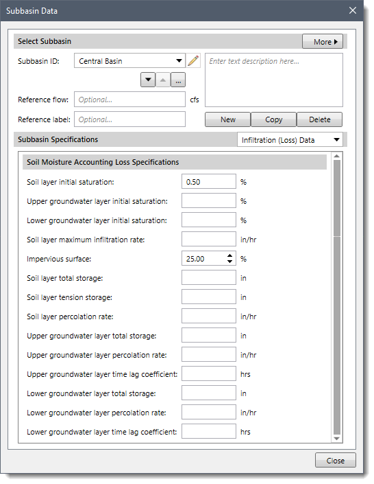
Infiltration (Loss) Data panel for Soil Moisture Accounting Loss method

The following input parameters are provided in the data panel:

Soil layer initial saturation
This entry field is used to specify the initial condition of the soil as the percentage of the soil that is full of water at the beginning of the simulation.
Upper/Lower groundwater layer initial saturation
These entry fields are used to specify the initial condition of the upper and lower groundwater layers.
Soil layer maximum infiltration rate
This entry field is used to set the upper bound on infiltration from the surface storage into the soil. If a surface storage method is selected, the actual infiltration in a particular time interval is a linear function of the surface and soil storage. If no surface storage method is selected, water will always infiltrate at the maximum rate.
Impervious surface
This entry field is used to specify the percentage of the subbasin area which is impervious.
Soil layer total storage
This entry field specifies the total storage available in the soil layer. Provide a zero value if you wish to eliminate soil calculations and pass infiltrated water directly to groundwater.
Soil layer tension storage
This entry field specifies the amount of water storage in the soil that does not drain under the effects of gravity. Percolation from the soil layer to the upper groundwater layer will occur whenever the current soil storage exceeds the tension storage. Water in tension storage is only removed by evapotranspiration. Tension storage must be less than soil storage.
Soil layer percolation rate
This entry field specifies the upper bound on percolation from the soil storage into the upper groundwater. The actual percolation rate is a linear function of the current storage in the soil and the current storage in the upper groundwater.
Upper groundwater layer total storage
This entry field specifies the total storage in the upper groundwater layer. It may be zero if you wish to eliminate the upper groundwater layer and pass water percolated from the soil directly to the lower groundwater layer.
Upper groundwater layer percolation rate
This entry field specifies the upper bound on percolation from the upper groundwater layer into the lower groundwater layer. The actual percolation rate is a linear function of the current storage in the upper and lower groundwater layers.
Upper groundwater layer time lag coefficient
This entry field specifies the time lag on a linear reservoir whereby water in storage becomes lateral outflow. The lateral outflow is available to become baseflow.
Lower groundwater layer total storage
This entry field specifies the total storage in the lower groundwater layer. It may be zero if you wish to eliminate the lower groundwater layer and pass water percolated from the upper groundwater layer directly to deep percolation.
Lower groundwater layer percolation rate
This entry field specifies the upper bound on deep percolation out of the system. The actual percolation rate is a linear function of the current storage in the lower groundwater layer.
Lower groundwater layer time lag coefficient
This entry field specifies the time lag on a linear reservoir whereby water in storage becomes lateral outflow. It is usually larger than the Upper groundwater layer time lag coefficient. The lateral outflow is likewise available to become baseflow.

Infiltration Methods along with the Kinematic Wave Runoff Method

When Kinematic Wave is selected for the Runoff (Transform) Method, two surface area sections are shown in the Infiltration (Loss) Data panel for defining data of the infiltration method. These include one for impervious surfaces and the other for pervious surfaces within the subbasin.

Below is an example of the Infiltration (Loss) Data panel displayed for the SCS Curve Number method.
SCS Curve Number method along with Kinematic Wave runoff method

Pros and Cons of Infiltration Methods

Method	Pros	Cons
Deficit and Constant	It is a mature method and easy to set up. The method is parsimonious as it includes few parameters to explain the variation of runoff volume. The method is scalable in that it allows for continuous simulation	Difficult to apply to ungauged areas due to lack of direct physical relationship of parameters and watershed properties. Models may be too simple to predict losses within an event.
Exponential	The method performs better in catching the sequential peaks since the loss rate is not constant and is represented by a decaying logarithmic function.	The method cannot be used for continuous simulation. There is no evapotranspiration component.
Green and Ampt	It is suitable to be used in ungauged catchments after obtaining information on soils.	The method is not widely adopted and hence considered less mature.
Layered Green and Ampt	This method can simulate water infiltration in fine-textured soil with a coarse interlayer.	Complex to use.
SCS Curve Number	This method relies only on one parameter that varies as a function of soil group, land use and treatment, and antecedent moisture conditions. A relatively simple, predictable and stable method.	The method does not account for the intensity of the rainfall.. The model's predicted values do not agree with the classical unsaturated flow theory. Infiltration rate will approach zero during a storm of a long duration, rather than constant rate as expected.
Initial and Constant	It is a mature method with successful applications across the world. Easy to set up This model is lean, with only a few parameters required to explain the variation in runoff volume.	This method is difficult to apply in ungauged watersheds. This method is too simple to predict losses within an event simulation.
Smith Parlange	The method is less likely to overestimate the infiltration early during a storm event. The method can adjust the infiltration process according to the temperature.	Complex to use. It is not suitable for continuous simulation.
Soil Moisture Accounting Loss	The method can simulate the dynamic movement of water in and above the soil by using five layers, i.e., canopy interception, surface depression storage, soil, upper groundwater, and lower groundwater.	There are challenges in parameter estimation and calibration.