
Welcome to CivilGEO Knowledge Base
Welcome to CivilGEO Knowledge Base
The HEC‑RAS bridge computations allow the modeler to analyze a bridge using several different methods without changing the bridge geometry.
The bridge computational methods have the ability to model:
This article describes how the HEC‑RAS program models bridge low flow conditions.
Low flow exists when the flow going through the bridge opening is open channel flow (water surface below the highest point on the low chord of the bridge opening). For low flow computations, the program first uses the momentum equation to identify the class of flow. This is accomplished by first calculating the momentum at critical depth inside the bridge at the upstream and downstream ends. The end with the higher momentum (therefore most constricted cross section) will be the controlling cross section in the bridge. If the two cross sections are identical, the program selects the upstream bridge cross section as the controlling cross section.
The momentum at critical depth in the controlling cross section is then compared to the momentum of the flow downstream of the bridge when performing a subcritical profile (upstream of the bridge for a supercritical profile).
The low flow is then classified according to the following criteria:
Class A low flow exists when the water surface through the bridge is completely subcritical (i.e., above critical depth). Energy losses through the expansion (cross sections 2 to 1) are calculated as friction losses and expansion losses. Friction losses are based on a weighted friction slope multiplied by the weighted reach length between cross sections 1 and 2. The weighted friction slope is based on one of the four available alternatives in HEC‑RAS, with the average conveyance method being the default. This option is user selectable. The average length used in the calculation is based on a discharge‑weighted reach length. Energy losses through the contraction (cross sections 3 to 4) are calculated as friction losses and contraction losses. Friction and contraction losses between cross sections 3 and 4 are calculated in the same way as friction and expansion losses between cross sections 1 and 2.
There are four methods available for computing losses through the bridge (cross sections 2 to 3):
The user can select any or all of these loss methods to compute bridge energy losses. This allows the modeler to compare the answers from several techniques all in a single execution of the program. If more than one method is selected, the user must choose either a single method as the final solution or direct the program to use the method that computes the greatest energy loss through the bridge as the final solution at cross section 3. Minimal results are available for all the methods computed, but detailed results are available for the method that is selected as the final answer. A detailed discussion of each method follows.
The energy‑based method treats a bridge in the same manner as a natural river cross section, except the area of the bridge below the water surface is subtracted from the total area, and the wetted perimeter is increased where the water is in contact with the bridge structure. As described previously, the program formulates two cross sections inside the bridge by combining the ground information of cross sections 2 and 3 with the bridge geometry. As shown in the figure below, for the purposes of discussion, these cross sections will be referred to as cross sections BD (Bridge Downstream) and BU (Bridge Upstream).
The sequence of calculations starts with a standard step calculation from just downstream of the bridge (cross section 2) to just inside of the bridge (cross section BD) at the downstream end. The program then performs a standard step through the bridge (from cross section BD to cross section BU). The last calculation is to step out of the bridge (from cross section BU to cross section 3).
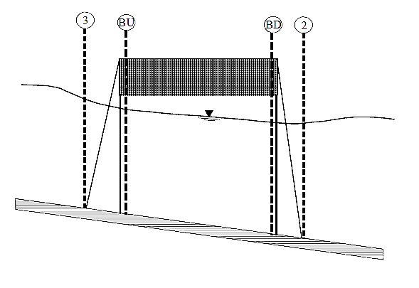
Figure 1: Cross sections near and inside the bridge
The energy‑based method requires Manning’s n values for friction losses and contraction and expansion coefficients for transition losses. The estimate of Manning’s n values is well documented in many hydraulics text books, as well as several research studies. Detailed output is available for cross sections inside the bridge (cross sections BD and BU) as well as the user defined cross sections (cross sections 2 and 3).
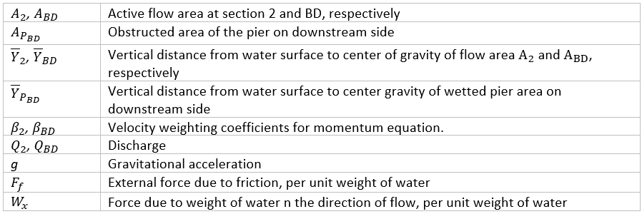
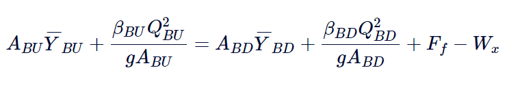
The momentum method is based on performing a momentum balance from cross section 2 to cross section 3. The momentum balance is performed in three steps. The first step is to perform a momentum balance from cross section 2 to cross section BD inside the bridge. The equation for this momentum balance is as follows:
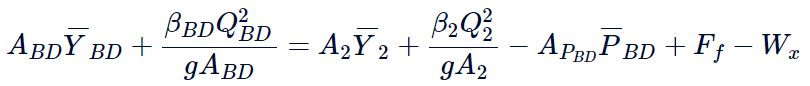
Where:
The second step is a momentum balance from cross section BD to BU (see Figure 1). The equation for this step is as follows:
The final step is a momentum balance from section BU to section 3 (see Figure 1). The equation for this step is as follows:
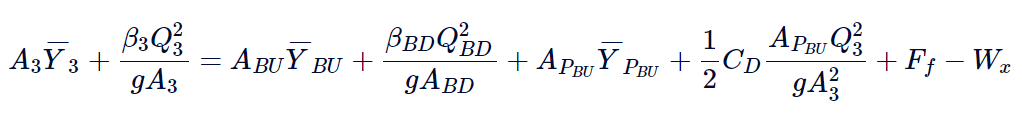
Where: CD = α1 and β1 coefficient for flow going around the piers.
Guidance on selecting drag coefficients can be found in Table 1 below.
The momentum balance method requires the use of roughness coefficients for the estimation of the friction force and a drag coefficient for the force of drag on piers. Drag coefficients are used to estimate the force due to the water moving around the piers, the separation of the flow, and the resulting wake that occurs downstream. Drag coefficients for various cylindrical shapes have been derived from experimental data (Lindsey, 1938). The following table shows some typical drag coefficients that can be used for piers:
Table 1: Typical Drag Coefficients for Various Pier Shapes
| Pier Shape | Pier Drag Coefficient CD |
|---|---|
| Circular pier | 1.20 |
| Elongated piers with semi-circular ends | 1.33 |
| Elliptical piers with 2:1 length to width | 0.60 |
| Elliptical piers with 4:1 length to width | 0.32 |
| Elliptical piers with 8:1 length to width | 0.29 |
| Square nose piers | 2.00 |
| Triangular nose with 30° angle | 1.00 |
| Triangular nose with 60° angle | 1.39 |
| Triangular nose with 90° angle | 1.60 |
| Triangular nose with 120° angle | 1.72 |
The momentum method provides detailed output for the cross sections inside the bridge (BU and BD) as well as outside the bridge (2 and 3). The user has the option of turning the friction and weight force components off. The default is to include the friction force but not the weight component. The computation of the weight force is dependent upon computing a mean bed slope through the bridge. Estimating a mean bed slope can be very difficult with irregular cross section data. A bad estimate of the bed slope can lead to large errors in the momentum solution. The user can turn the weight force on if he or she feels that the bed slope through the bridge is well behaved for their project.
During the momentum calculations, if the water surface (at cross sections BD and BU) comes into contact with the maximum low chord of the bridge, the momentum balance is assumed to be invalid and the results are not used.
The Yarnell equation is an empirical equation that is used to predict the change in water surface from just downstream of the bridge (cross section 2 of Figure 1) to just upstream of the bridge (cross section 3). The equation is based on approximately 2600 lab experiments in which the researchers varied the shape of the piers, the width, the length, the angle, and the flow rate. The Yarnell equation is as follows (Yarnell, 1934):
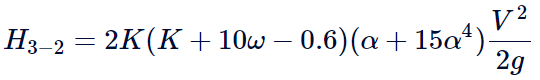
Where:
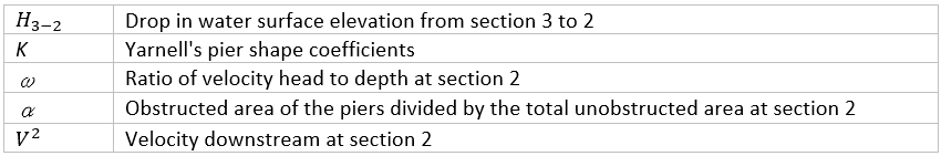
The computed upstream water surface elevation (cross section 3) is simply the downstream water surface elevation plus H3‑2. With the upstream water surface known, the program computes the corresponding velocity head and energy elevation for the upstream section (cross section 3). When the Yarnell method is used, hydraulic information is only provided at cross sections 2 and 3 (no information is provided for cross sections BU and BD).
The Yarnell equation is sensitive to the pier shape (K coefficient), the pier obstructed area, and the velocity of the water. The method is not sensitive to the shape of the bridge opening, the shape of the abutments, or the width of the bridge. Because of these limitations, the Yarnell method should only be used at bridges where the majority of the energy losses are associated with the piers. When Yarnell’s equation is used for computing the change in water surface through the bridge, the user must supply the Yarnell pier shape coefficient, K.
The following table provides values for the Yarnell pier coefficient for various pier shapes:
Table 2: Yarnell pier coefficient, K, for various pier shapes
| Pier Shape | Yarnell K Coefficient |
|---|---|
| Semi-circular nose and tail | 0.90 |
| Twin-cylinder piers with connecting diaphragm | 0.95 |
| Twin-cylinder piers without diaphragm | 1.05 |
| 90 degree triangular nose and tail | 1.05 |
| Square nose and tail | 1.25 |
| Ten pile trestle bent | 2.50 |
The low flow hydraulic computations of the Federal Highway Administration’s (FHWA) WSPRO computer program has been adapted as an option for low flow hydraulics in HEC‑RAS. The WSPRO methodology has been modified slightly in order to fit into the HEC‑RAS concept of cross section locations around and through a bridge.
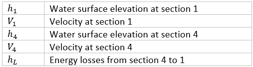
The WSPRO method computes the water surface profile through a bridge by solving the energy equation. The method is an iterative solution performed from the exit cross section (1) to the approach cross‑section (4). The energy balance is performed in steps from the exit cross section (1) to the cross section just downstream of the bridge (2); from just downstream of the bridge (2) to inside of the bridge at the downstream end (BD); from inside of the bridge at the downstream end (BD) to inside of the bridge at the upstream end (BU); From inside of the bridge at the upstream end (BU) to just upstream of the bridge (3); and from just upstream of the bridge (3) to the approach cross section (4). A general energy balance equation from the exit cross section to the approach cross section can be written as follows:
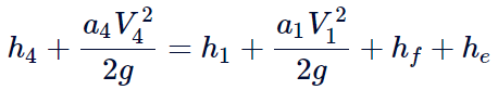
Where:
The incremental energy losses from cross section 4 to 1 are calculated as follows:
Losses from cross section 1 to cross section 2 are based on friction losses and an expansion loss. Friction losses are calculated using the geometric mean friction slope times the flow weighted distance between cross sections 1 and 2. The following equation is used for friction losses from cross sections 1 to 2:
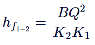
Where B is the flow weighted distance between cross sections 1 and 2, and K1 and K2 are the total conveyance at cross sections 1 and 2 respectively. The expansion loss from cross section 2 to cross section 1 is computed by the following equation:
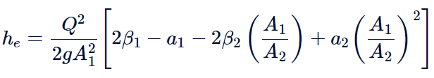
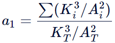
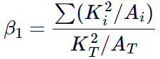
Where α and β are energy and momentum correction factors for non-uniform flow. α1 and β1 are computed as follows:
α2 and β2 are related to the bridge geometry and are defined as follows:
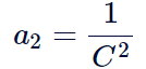
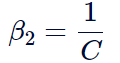
Where C is an empirical discharge coefficient for the bridge, which was originally developed as part of the Contracted Opening method by Kindswater, Carter, and Tracy (USGS, 1953), and subsequently modified by Matthai (USGS, 1968).
Losses from cross section 2 to cross section 3 are based on friction losses only. The energy balance is performed in three steps: from cross section 2 to BD; BD to BU; and BU to 3. Friction losses are calculated using the geometric mean friction slope times the flow weighted distance between cross sections. The following equation is used for friction losses from BD to BU:
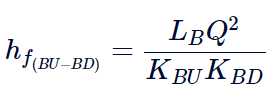
Where KBU and KBD are the total conveyance at cross sections BU and BD respectively, and LB is the length through the bridge. Similar equations are used for the friction losses from cross section 2 to BD and BU to 3.
Energy losses from cross section 3 to cross section 4 are based on friction losses only. The equation for computing the friction loss is as follows:
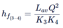
Where Lav is the effective flow length in the approach reach, and K3 and K4 are the total conveyances at cross sections 3 and 4. The effective flow length is computed as the average length of 20 equal conveyance stream tubes (FHWA, 1986).
Class B low flow can exist for either subcritical or supercritical profiles. For either profile, class B flow occurs when the profile passes through critical depth in the bridge constriction. For a subcritical profile, the momentum equation is used to compute an upstream water surface (cross section 3) above critical depth and a downstream water surface (cross section 2) below critical depth. For a supercritical profile, the bridge is acting as a control and is causing the upstream water surface elevation to be above critical depth. Momentum is used to calculate an upstream water surface above critical depth and a downstream water surface below critical depth. If for some reason the momentum equation fails to converge on an answer during the class B flow computations, the program will automatically switch to an energy‑based method for calculating the class B profile through the bridge.
Whenever class B flow is found to exist, the user should run the program in a mixed flow regime mode. If the user is running a mixed flow regime profile, the program will proceed with backwater calculations upstream, and later with forewater calculations downstream from the bridge. Also, any hydraulic jumps that may occur upstream and downstream of the bridge can be located if they exist.
Class C low flow exists when the water surface through the bridge is completely supercritical. The program can use either the energy equation or the momentum equation to compute the water surface through the bridge for this class of flow.


CivilGEO G2 Reviews
4.8/5.0 Rating, Over 230 Reviews

GeoHECRAS is recognized as the top Civil Engineering Design Software with an average of 4.8 out of 5.0 rating from over 230 real user reviews on G2.


We use cookies to give you the best online experience. By agreeing you accept the use of cookies in accordance with our cookie policy.
When you visit any web site, it may store or retrieve information on your browser, mostly in the form of cookies. Control your personal Cookie Services here.


