
Welcome to CivilGEO Knowledge Base
Welcome to CivilGEO Knowledge Base
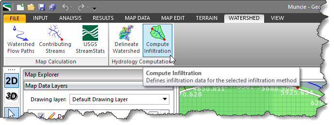
In GeoHECRAS, the Compute Infiltration command allows the user to define the precipitation infiltration method (i.e., SCS Curve Number, Green and Ampt, or Deficit Constant) to be used for computing the 2D surface losses from a storm event.
Follow the steps below to use the Compute Infiltration command:
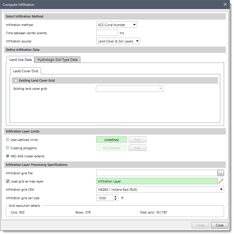
The following sections describe the Compute Infiltration command and how to interact with the above dialog box.
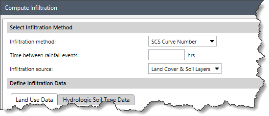
The Select Infiltration Method section allows the user to define the infiltration method to be used for computations.
The Define Infiltration Data section contains two panels: Land Use Data and Hydrologic Soil Type Data. These panels are used to define the infiltration parameters for computing the various infiltration methods. Based upon the option selected in the Infiltration source combo box entry in the Select Infiltration Method section, the contents of this section will be modified accordingly.
Note that if the Land Cover & Soil Layers option is selected as the infiltration source, then the Land Use Data panel, as shown below, will be similar for all three infiltration methods (i.e., Deficit and Constant, Green and Ampt, SCS Curve Number).
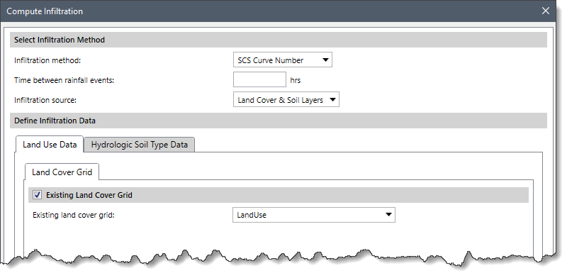
The Land Use Data panel allows the user to describe the land use data. This panel contains the following subpanels:
The Land Cover Grid subpanel allows the user to select an existing land cover grid. The Existing land cover grid dropdown combo box contains all the land cover grids added to the project.
The Hydrologic Soil Type Data panel allows the user to describe the soil grid data.
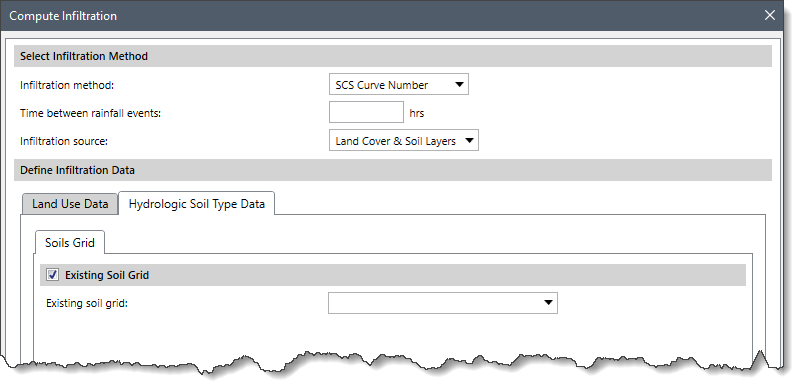
This panel contains the following subpanel:
The Soil Grid subpanel allows the user to select an existing soil grid. The Existing soil grid dropdown combo box contains all the soil grids added to the project.
If the user selects the Shapefile Layer option as an infiltration source in the Select Infiltration Method section, the contents of the Compute Infiltration dialog box will be changed as shown below.
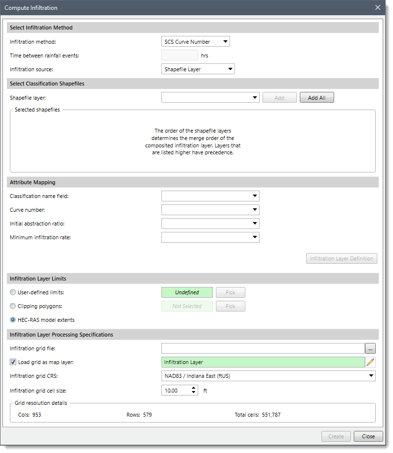
The Select Classification Shapefile section controls the selection of shapefile layers to be used for computing the infiltration. In this section, the user can add already loaded shapefiles using the Shapefile layer dropdown combo box.
From the Shapefile layer dropdown combo box, select the shapefile layers, one at a time, and click the [Add] button. The selected shapefile(s) will be added to the Selected shapefiles grid. Alternatively, click the [Add All] button to add all the shapefiles available in the project.
To change the order of the added shapefile(s) in the grid, select the appropriate row and right-click to display a context menu. Then, select the Move Layer Up or Move Layer Down context menu command to change the order of the highlighted shapefile layer. Alternatively, select the up or down arrows option adjacent to the highlighted layer to change the layer order.
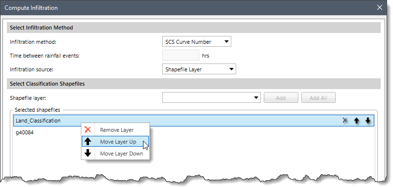
Note that shapefile layers that are higher in the listing have precedence over layers that appear lower in the list.
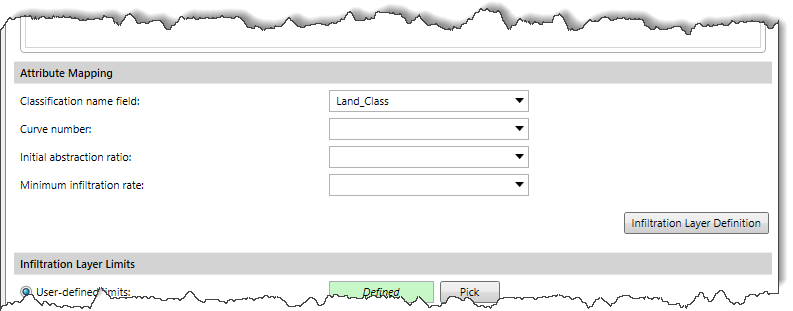
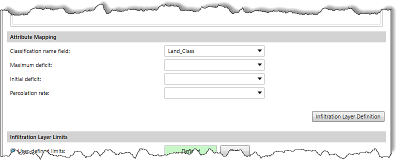
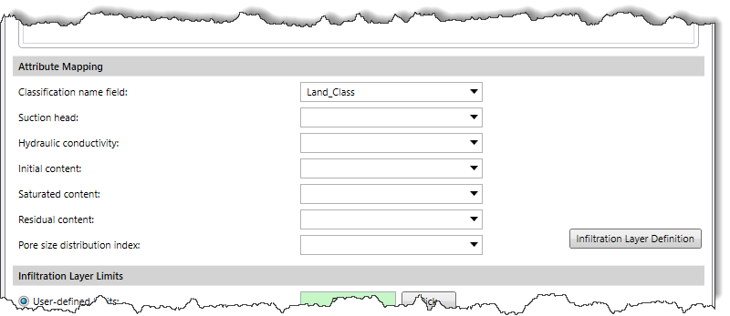
This section allows the user to select the corresponding shapefile fields to map to the required attributes. Based upon the infiltration method selected in the Select Infiltration Method section, the dropdown entries contained in this section will be changed.
The following dropdown combo box attribute entries are provided when the SCS Curve Number option is selected as an infiltration method in the Select Infiltration Method section.
The following dropdown combo box attribute entries are provided when the Deficit Constant option is selected as an infiltration method in the Select Infiltration Method section.
The following dropdown combo box attribute entries are provided when the Green and Ampt option is selected as an infiltration method in the Select Infiltration Method section.
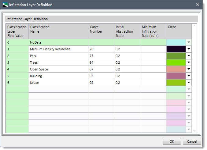
The user can define various mapped parameters using the [Infiltration Layer Definition] button. Clicking on this button will display the Infiltration Layers Definition dialog box specific to the infiltration method selected.
This section allows the user to define the limits of the infiltration layer to be generated.
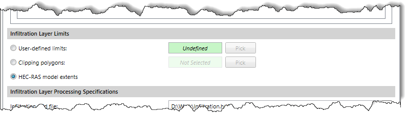
The following options are provided:
This section details how the infiltration layer data should be processed.
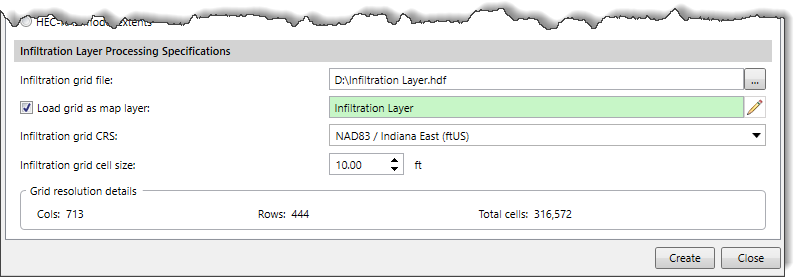
The Infiltration grid file entry is used to define the name and the directory address where the infiltration layer grid file will be saved.
The Load grid as map layer checkbox option causes the software to add the infiltration grid as a layer in the Map Data Layers panel. By default, this checkbox option is checked. The software automatically defines the name of the map data layer based on the infiltration grid file name provided by the user. However, the user can edit the map layer name using the edit tool present next to the Load grid as map layer entry field.
The Infiltration grid CRS dropdown combo box allows the user to define the layer’s CRS (Coordinate Reference System). If there is only one CRS in the project, the software automatically selects it.
The Infiltration grid cell size spin control button allows the user to manually define the grid cell size. The finer the grid resolution (or smaller the cell size) defined, the greater the detail that can be represented in the infiltration grid. By default, the software uses a value of 10 ft.
Based on the defined grid cell size and the extent of the infiltration layer, the Grid resolution details pane displays the total number of cells and the number of columns and rows that the infiltration layer grid file will contain.
After defining the required infiltration parameters in the Compute Infiltration dialog box, click the [Create] button. The software will then combine the source infiltration layers to create a single composite infiltration layer grid file. This layer will be an HDF file created by the intersection of the different land use and soil group data polygons, thereby creating sub-polygons containing a corresponding land use and soil group.
In the Map Data Layers panel, the software provides a data legend for each created infiltration layer that lists the infiltration data included within that layer. The user can expand the layer to view the data legend.
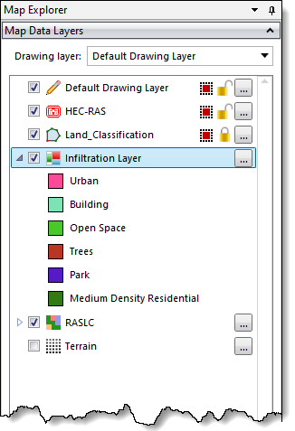
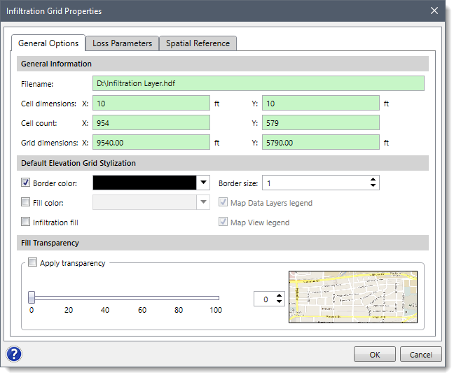
Clicking on the […] button adjacent to the created Infiltration Layer will display the Infiltration Grid Properties dialog box, allowing the user to define the color and style of the infiltration layers.


CivilGEO G2 Reviews
4.8/5.0 Rating, Over 230 Reviews

GeoHECRAS is recognized as the top Civil Engineering Design Software with an average of 4.8 out of 5.0 rating from over 230 real user reviews on G2.


We use cookies to give you the best online experience. By agreeing you accept the use of cookies in accordance with our cookie policy.
When you visit any web site, it may store or retrieve information on your browser, mostly in the form of cookies. Control your personal Cookie Services here.


